Data generation • gmwmx2

This vignette shows how to build stochastic models, combine them with +, generate data, and plot the results.

library(gmwmx2)
set.seed(123)

Available models

You can build a single stochastic process with any of the following model constructors:

wn() (white noise)
ar1() (AR(1))
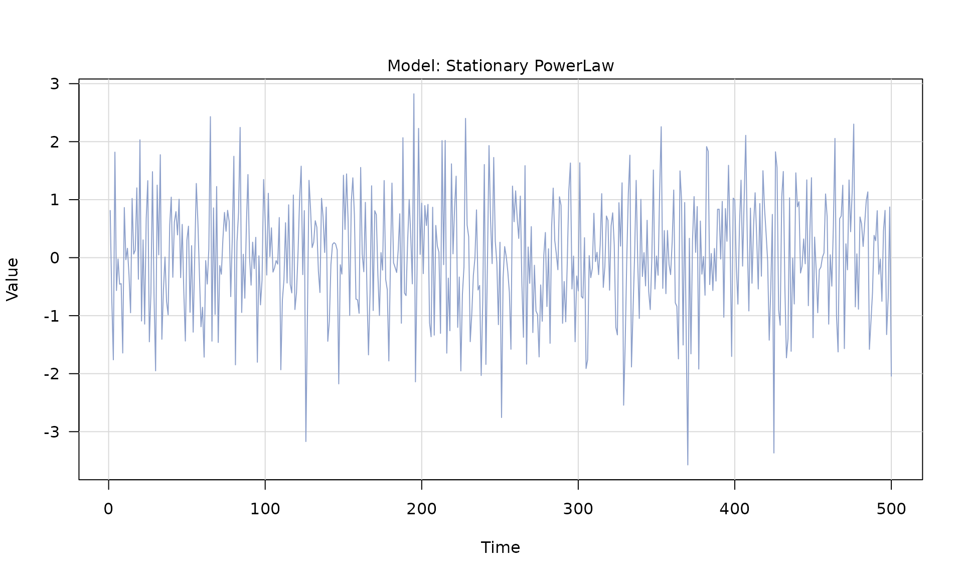
pl() (power-law)
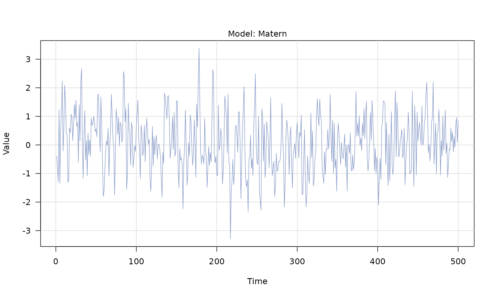
matern() (Matérn)
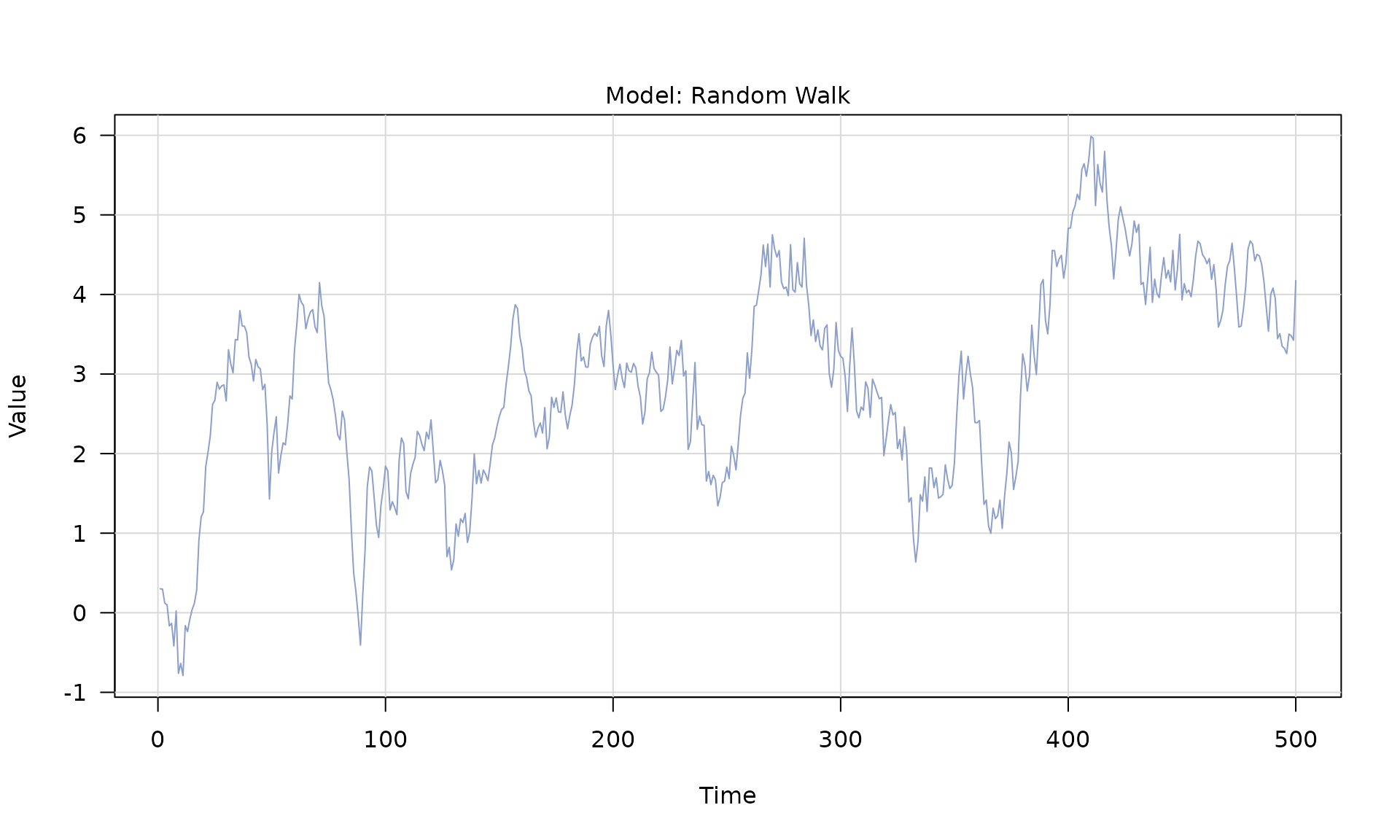
rw() (random walk)
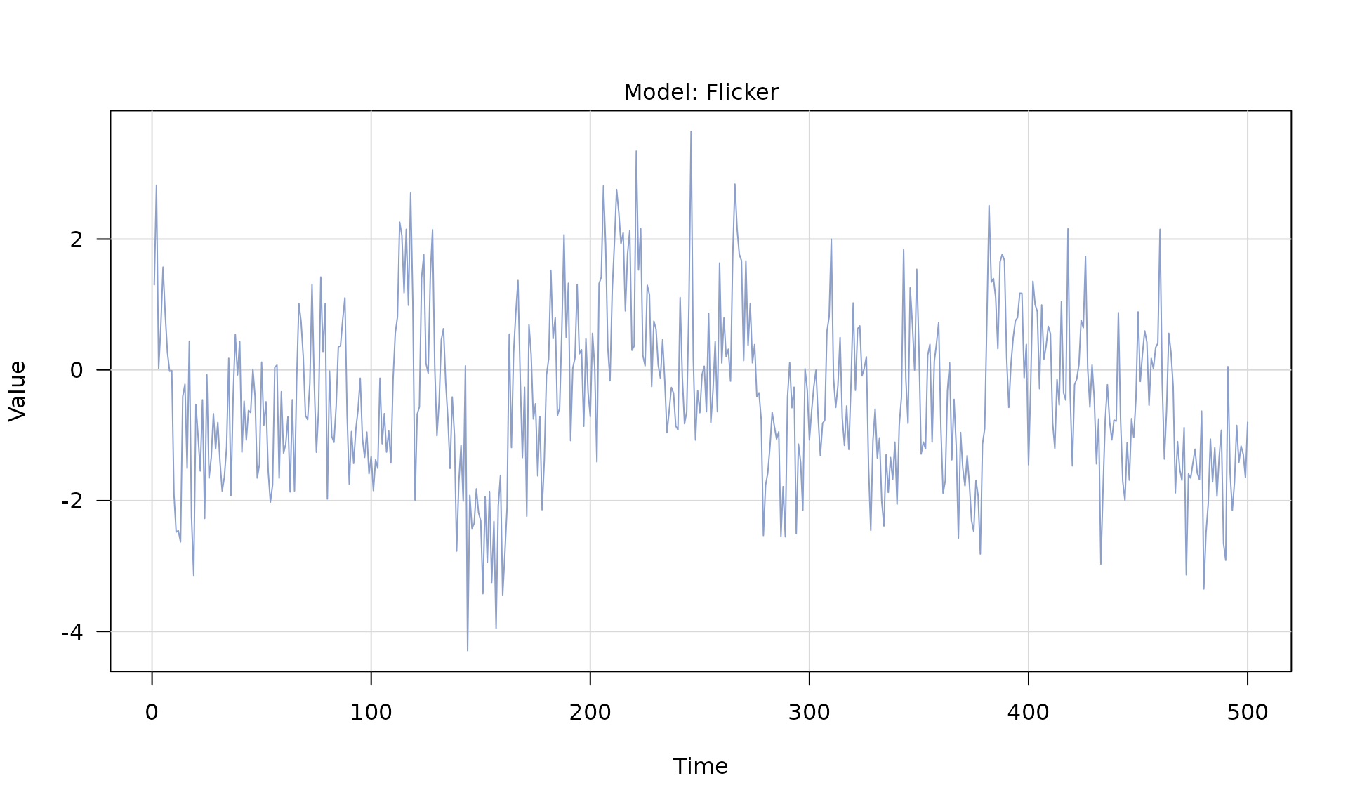
flicker() (flicker)

Each constructor returns a time_series_model object that can be plotted or combined with others using +.

Stochastic models

White noise

model_wn <- wn(sigma2 = 1)
series_wn <- generate(model_wn, n = 500)
plot(series_wn)

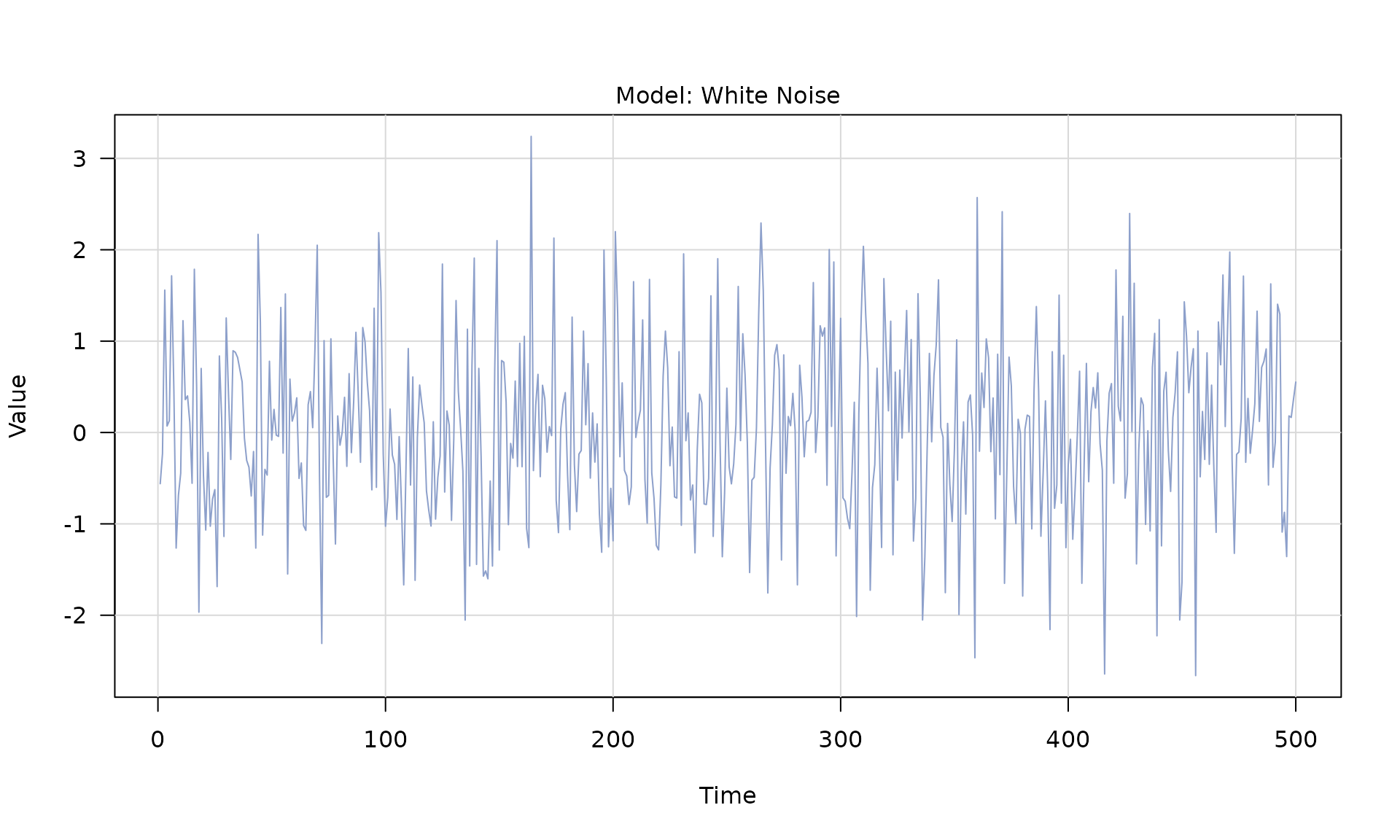The generated object is a generated_time_series with a numeric series in $series:

head(series_wn$series)

## [1] -0.56047565 -0.23017749  1.55870831  0.07050839  0.12928774  1.71506499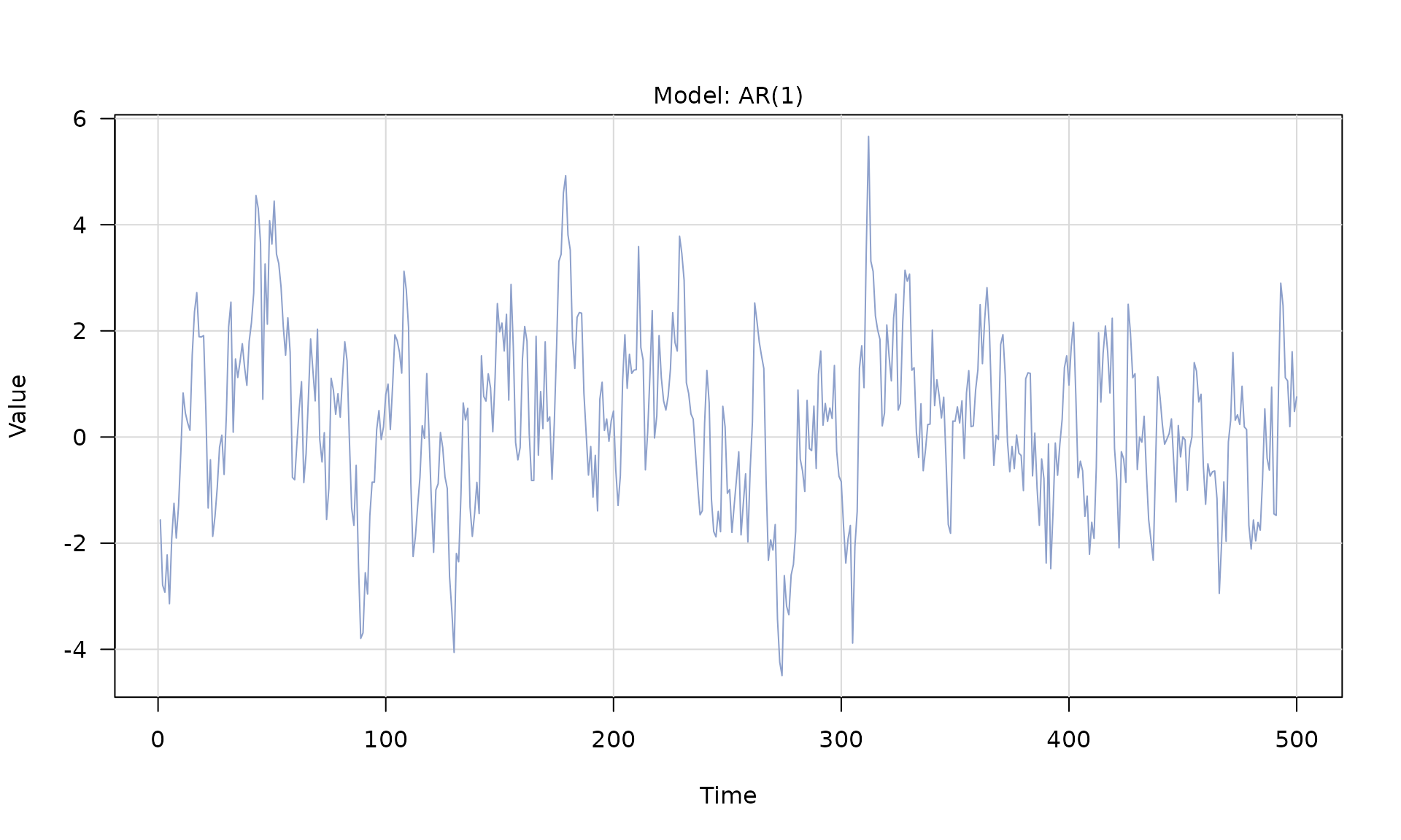

AR(1)

model_ar1 <- ar1(phi = 0.8, sigma2 = 1)
series_ar1 <- generate(model_ar1, n = 500)
plot(series_ar1)

Power-law

model_pl <- pl(kappa = 0.3, sigma2 = 1)
series_pl <- generate(model_pl, n = 500)
plot(series_pl)

Matérn

model_matern <- matern(sigma2 = 1, lambda = 1, alpha=1)
series_matern <- generate(model_matern, n = 500)
plot(series_matern)

Random walk

model_rw <- rw(sigma2 = 0.1)
series_rw <- generate(model_rw, n = 500)
plot(series_rw)

Flicker

model_fl <- flicker(sigma2 = 1)
series_fl <- generate(model_fl, n = 500)
plot(series_fl)

Reproducible generation

You can set a random seed before calling generate(), or pass a seed directly to generate(), to make the output deterministic. Using the same seed and model parameters produces the exact same time series.

model_wn <- wn(sigma2 = 1)

set.seed(1234)
series_a <- generate(model_wn, n = 100)

series_b <- generate(model_wn, n = 100, seed = 1234)
series_c <- generate(model_wn, n = 100, seed = 4321)

all.equal(series_a$series, series_b$series)

## [1] TRUE

all.equal(series_a$series, series_c$series)

## [1] "Mean relative difference: 1.310458"

Composite models (sum of processes)

Use + to build a composite model from multiple stochastic processes. The result is a sum_model that can be passed to generate().

model_wn_ar1 <- wn(sigma2 = 1) + ar1(phi = 0.8, sigma2 = 0.5)
class(model_wn_ar1)

## [1] "sum_model"

series_wn_ar1 <- generate(model_wn_ar1, n = 500)
plot(series_wn_ar1)

The composite output is a generated_composite_model_time_series with:

series (the total sum)
components (a list of each component series)
n (length of the series)
model (names of each component)
parameters (parameters of each component)

names(series_wn_ar1)

## [1] "series"     "components" "n"          "model"      "parameters"