Plot method for a gmwm2_fit object

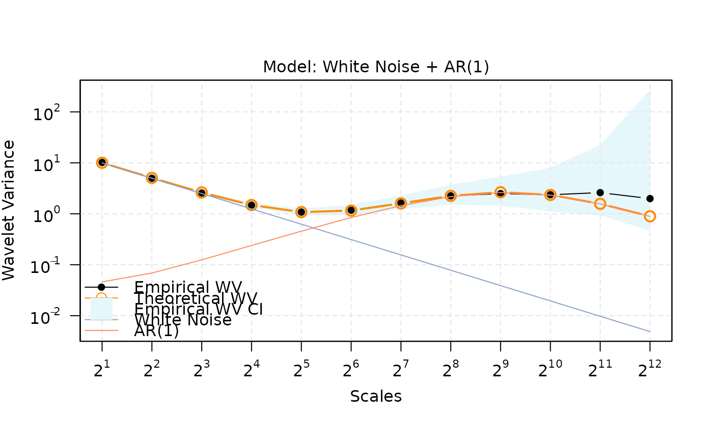
Plots empirical wavelet variance with the fitted theoretical curve and, for sum models, component-implied theoretical curves.

# S3 method for class 'gmwm2_fit'
plot(
  x,
  show_ci = TRUE,
  col_emp = "black",
  col_theo = "darkorange",
  col_ci = "#e6f7fb",
  lwd = 2,
  pch_emp = 16,
  pch_theo = 21,
  cex_theo = 1.4,
  legend_pos = "auto",
  ...
)

Arguments

x

A gmwm2_fit object.

show_ci

Logical; if TRUE and available, show empirical CI bars.

col_emp

Color for empirical WV points/line.

col_theo

Color for theoretical WV line.

col_ci

Color for empirical WV CI band.

lwd

Line width for theoretical curve.

pch_emp

Plotting character for empirical points.

pch_theo

Plotting character for theoretical points.

cex_theo

Size for theoretical points.

legend_pos

Legend position (e.g., "topleft") or "auto".

...

Additional arguments passed to plot().

Value

The input object, invisibly.

Examples

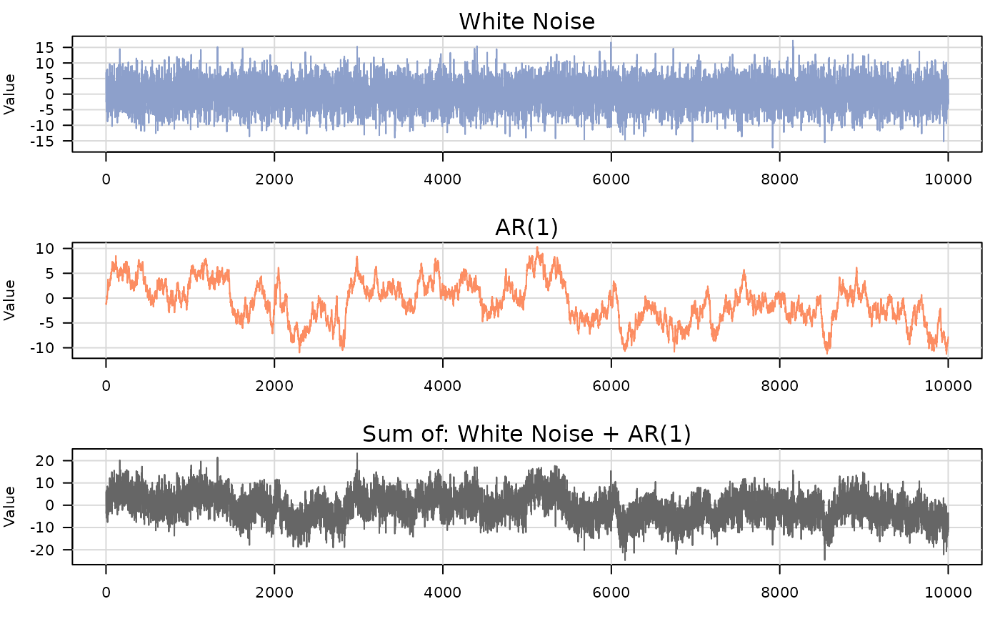
n = 10000
mod = wn(20) + ar1(phi = .995, sigma2 = .2)
y = generate(mod, n = n, seed = 123)
plot(y)

fit = gmwm2(y, model = wn() + ar1() )
fit
#> GMWM fit
#> 
#> Stochastic model
#>   Sum of 2 processes
#> 
#>   [1] White Noise
#>       Parameters : sigma2
#> 
#>   [2] AR(1)
#>       Parameters : phi, sigma2
#> 
#> 
#> Estimated parameters
#>   1) White Noise: sigma2 = 19.96
#>   2) AR(1): phi = 0.9933, sigma2 = 0.1838
#> 
#> Optimization
#>   Convergence : converged (code 0)
#>   Iterations  : 136
#>   Loss        : 0.07507
plot(fit)