Implements the Generalized Method of Wavelet Moments (GMWM) estimator
to fit a time_series_model, a sum_model or a numeric vector.
gmwm2(x, model, omega = NULL, method = "L-BFGS-B", control = list(), ...)Arguments
- x
Numeric vector, or a
generated_time_series/generated_composite_model_time_seriesobject (itsseriesis used).- model
A
time_series_modelorsum_model.- omega
Optional weighting matrix. If
NULL, a default based on the empirical WV confidence intervals is used.- method
Optimization method passed to
stats::optim.- control
Optional list of control parameters for
stats::optim.- ...
Additional arguments passed to
stats::optim.
Value
An object of class gmwm2_fit with elements:
theta_hat (real space), theta_domain (constrained space),
model, empirical_wvar, theoretical_wvar, optim, and n.
Details
The GMWM estimator solves a weighted least-squares criterion of the form
$$
\left\{\hat{\boldsymbol{\nu}} - \boldsymbol{\nu}(\boldsymbol{\theta})\right\}^{\top}
\boldsymbol{\Omega}
\left\{\hat{\boldsymbol{\nu}} - \boldsymbol{\nu}(\boldsymbol{\theta})\right\}
$$
where \(\hat{\boldsymbol{\nu}}\) denotes the empirical wavelet
variance and \(\boldsymbol{\nu}(\boldsymbol{\theta})\)
the corresponding theoretical wavelet variance implied by the model
parameters \(\boldsymbol{\theta}\). The weighting matrix
\(\boldsymbol{\Omega}\) defaults to a diagonal matrix with entries proportional to the
inverse squared width of the empirical WV asymptotic confidence intervals. Provide
omega to use a custom weighting (e.g., from a theoretical covariance).
References
Guerrier, S., Skaloud, J., Stebler, Y., and Victoria-Feser, M.-P. (2013). Wavelet-variance-based estimation for composite stochastic processes. Journal of the American Statistical Association, 108(503), 1021-1030. doi:10.1080/01621459.2013.799920.
Examples
n = 10000
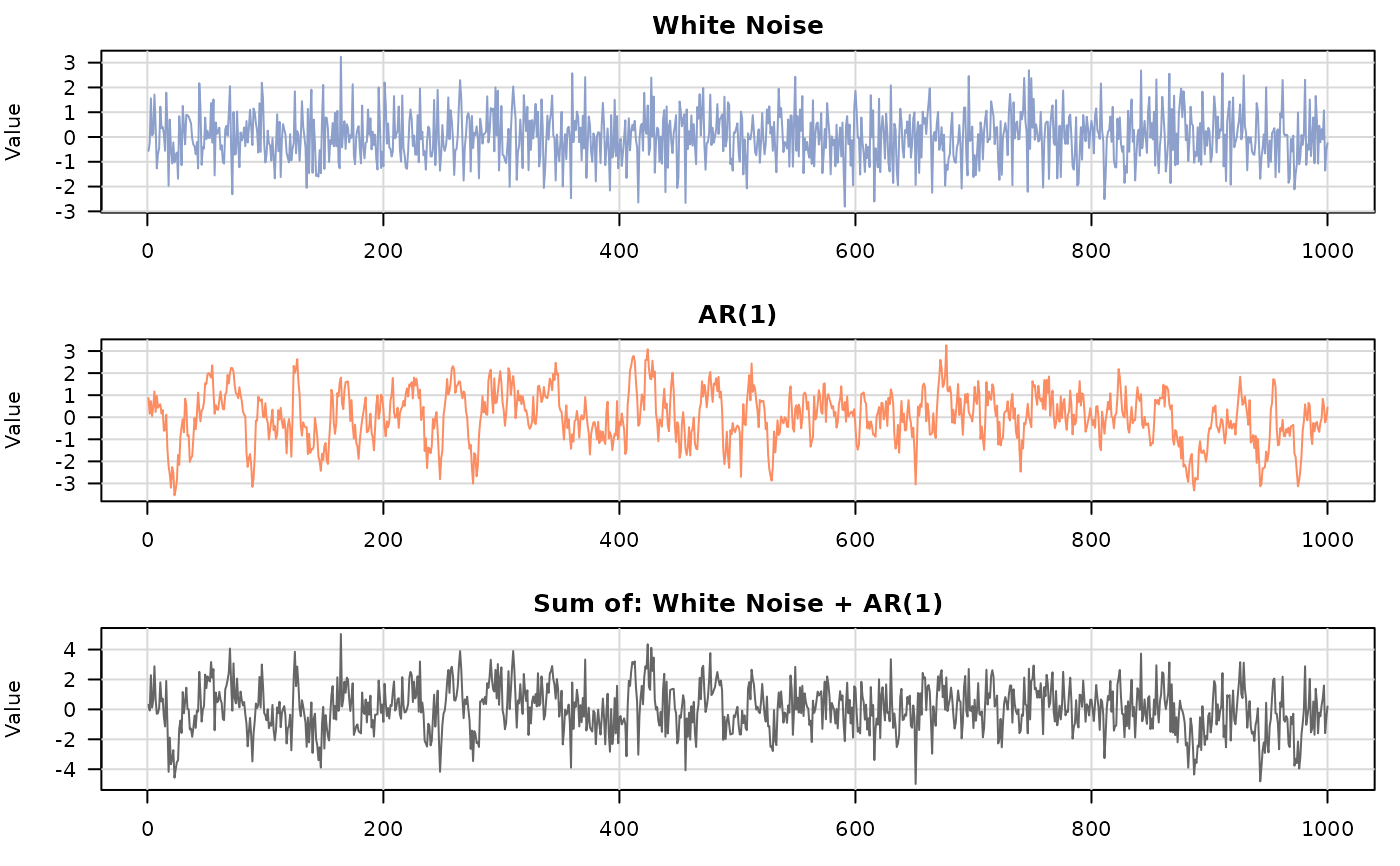
mod = wn(20) + ar1(phi = .995, sigma2 = .2)
y = generate(mod, n = n, seed = 123)
plot(y)
 fit = gmwm2(y, model = wn() + ar1())
fit
#> GMWM fit
#>
#> Stochastic model
#> Sum of 2 processes
#>
#> [1] White Noise
#> Parameters : sigma2
#>
#> [2] AR(1)
#> Parameters : phi, sigma2
#>
#>
#> Estimated parameters
#> 1) White Noise: sigma2 = 19.96
#> 2) AR(1): phi = 0.9933, sigma2 = 0.1838
#>
#> Optimization
#> Convergence : converged (code 0)
#> Iterations : 104
#> Loss : 0.07507
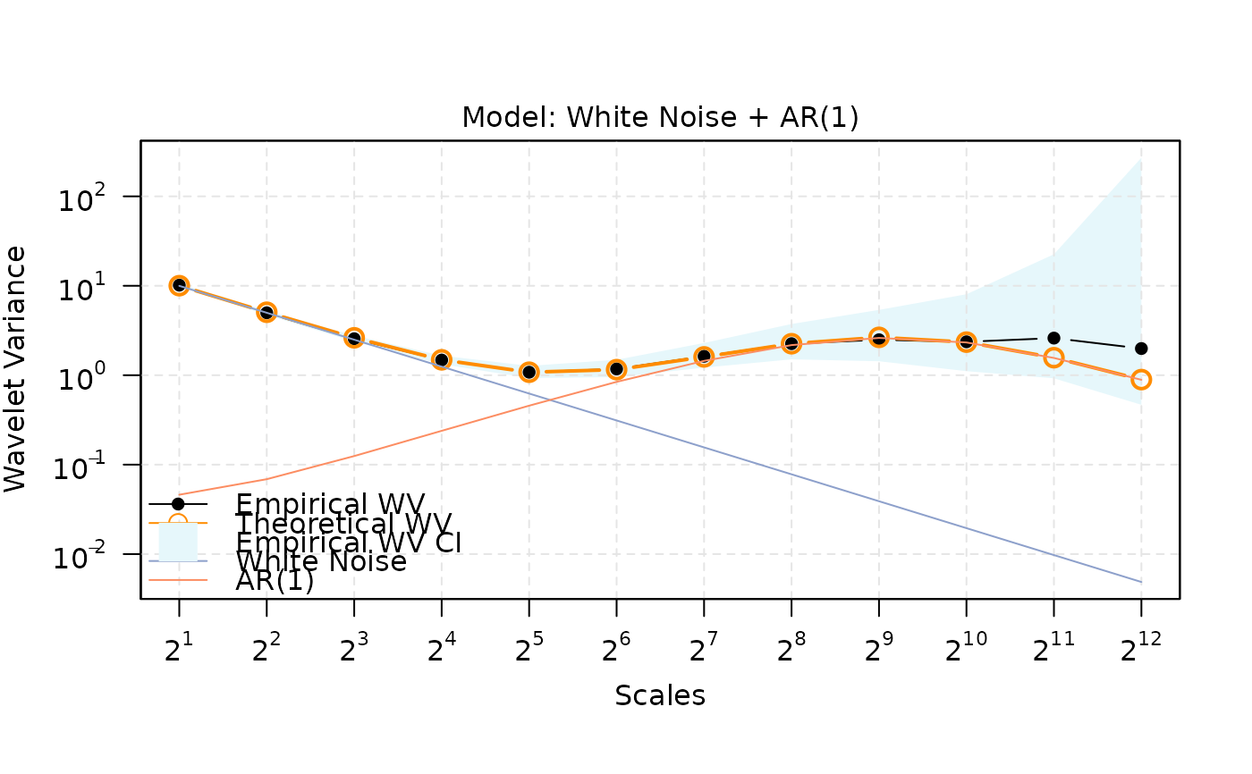
plot(fit)
fit = gmwm2(y, model = wn() + ar1())
fit
#> GMWM fit
#>
#> Stochastic model
#> Sum of 2 processes
#>
#> [1] White Noise
#> Parameters : sigma2
#>
#> [2] AR(1)
#> Parameters : phi, sigma2
#>
#>
#> Estimated parameters
#> 1) White Noise: sigma2 = 19.96
#> 2) AR(1): phi = 0.9933, sigma2 = 0.1838
#>
#> Optimization
#> Convergence : converged (code 0)
#> Iterations : 104
#> Loss : 0.07507
plot(fit)