GMWMX: Estimate linear models with dependent errors and missing observations
Source:vignettes/gmwmx2_new_w_missing.Rmd
gmwmx2_new_w_missing.RmdThis vignette demonstrate on to use the GMWMX estimator to estimate linear models with dependent errors described by a composite stochastic process in presence of missing observations. Consider the model defined as:
Missingness is modeled by a binary process with indicating observation, and a missing observation. The missingness process is independent of $ and respect the following definition: with expectation , for all , with covariance matrix whose structure is assumed known up to the parameter vector The observed series is
The design matrix with rows zeroed out for missing observations can be written as . The least‑squares estimator based on observed data is and we compute residuals .
We then estimate the parameters of the missingness process using maximum likelihood estimation, assuming a two state Markov model using the Maximum Likelihood Estimator.
We then estimate the stochastic parameters using the GMWM estimator:
$$\begin{equation} \hat{\boldsymbol{\gamma}} = \argmin_{\boldsymbol{\gamma} \in \boldsymbol{\Gamma}} \,\{\hat{\boldsymbol{\nu}} - \boldsymbol{\nu}(\boldsymbol{\gamma}, \hat{\boldsymbol{\vartheta}})\}^{\trans} \, \boldsymbol{\Omega} \, \{\hat{\boldsymbol{\nu}} - \boldsymbol{\nu}(\boldsymbol{\gamma}, \hat{\boldsymbol{\vartheta}})\}, \end{equation}$$
where is the estimated wavelet variance computed on the estimated residuals and is the pre-computed estimator of the parameter , with being any positive-definite matrix.
Overall, these examples illustrate how gmwmx2_new()
supports inference for linear regression models with dependent errors in
presence of missing observations, and how the results compare to a naive
OLS fit that ignores dependence.
library(gmwmx2)
library(wv)
library(dplyr)

boxplot_mean_dot <- function(x, ...) {
  boxplot(x, ...)
  x_mat <- as.matrix(x)
  mean_vals <- colMeans(x_mat, na.rm = TRUE)
  points(seq_along(mean_vals), mean_vals, pch = 16, col = "black")
}
We load the packages used for simulation, wavelet variance
diagnostics, and summary plots. The helper
boxplot_mean_dot() overlays Monte Carlo means on top of
each boxplot for easier comparison.
We first construct a design matrix with an intercept, linear trend, and annual seasonal components. This deterministic signal will be used across examples.
n = 10*365
X = matrix(NA, nrow = n, ncol = 4)
# intercept
X[, 1] = 1
# trend
X[, 2] = 1:n
# annual sinusoid
omega_1 <- (1 / 365.25) * 2 * pi
X[, 3] <- sin((1:n) * omega_1)
X[, 4] <- cos((1:n) * omega_1)
beta = c(1, 0.01, 2, 1.5)

# visualize the deterministic signal
plot(x = X[, 2], y = X %*% beta, type = "l",
     main = "Signal", xlab = "Time", ylab = "Signal")
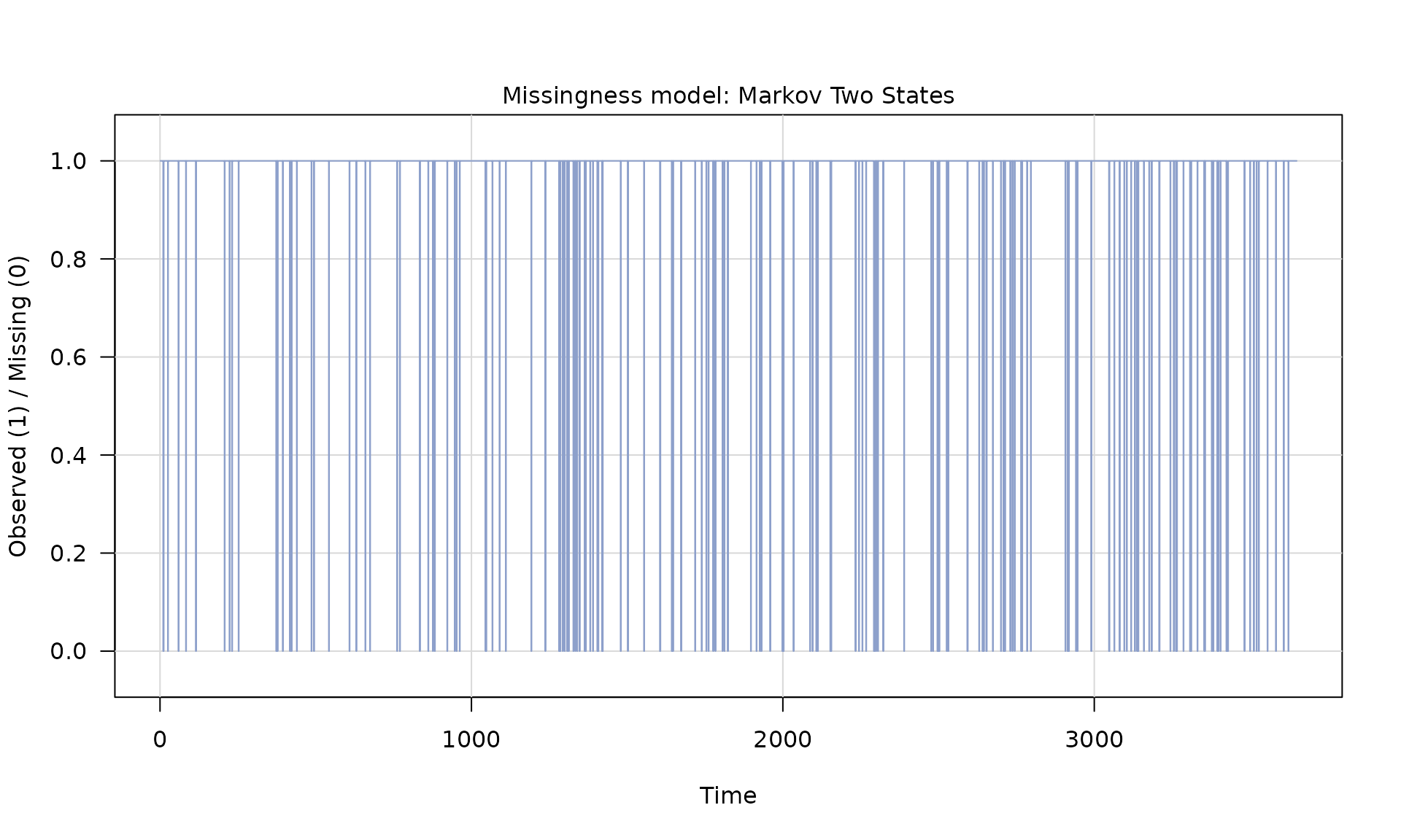
Next we simulate dependent errors, add them to the signal, and then
introduce missing observations using a two‑state Markov model. This is
the key difference from vignettes/gmwmx2_new.Rmd, which
uses fully observed data.
# Example 1: White noise + AR(1)
phi_ar1 = 0.95
sigma2_ar1 = 1
sigma2_wn = 1
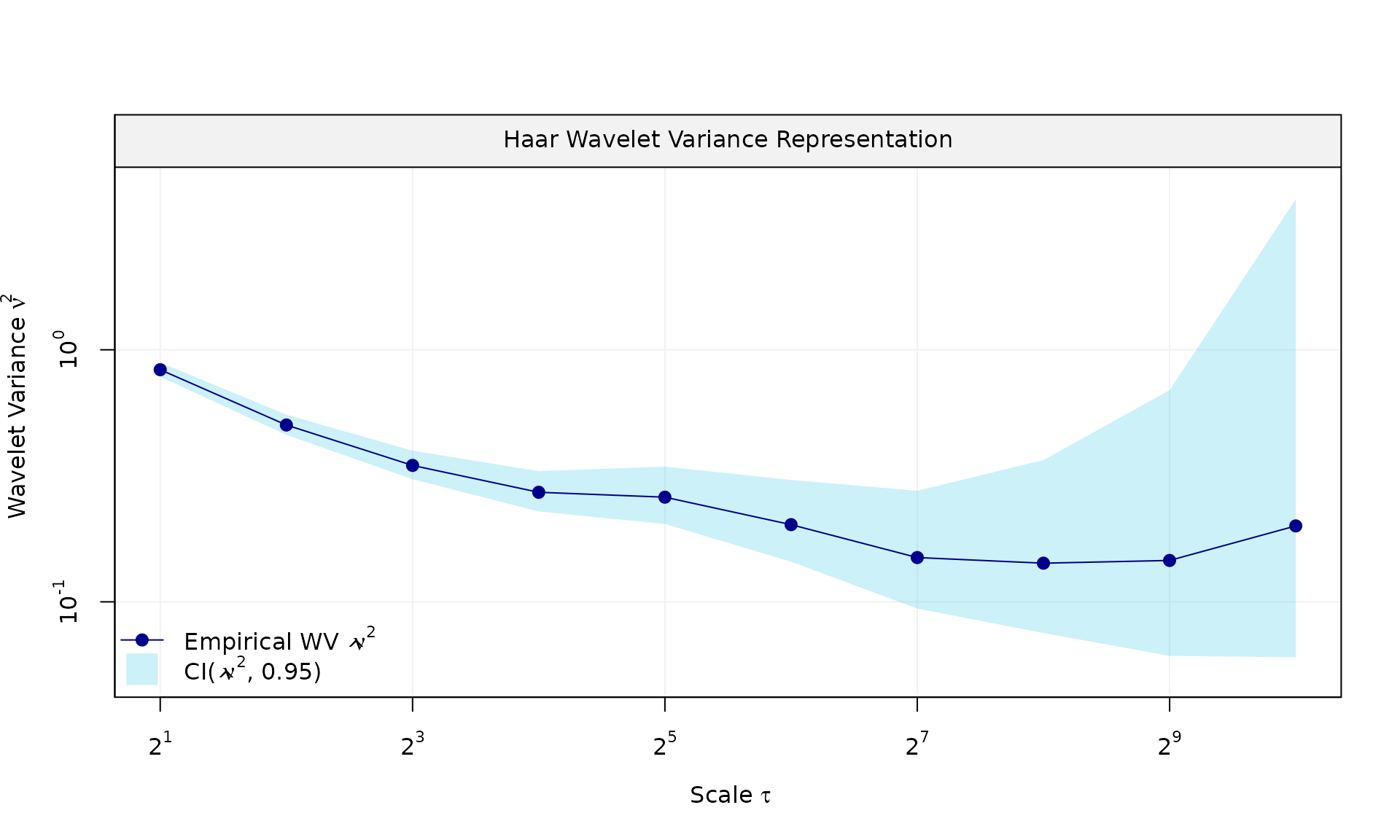
eps = generate(ar1(phi = phi_ar1, sigma2 = sigma2_ar1) + wn(sigma2_wn), n = n, seed = 123)$series
plot(wv::wvar(eps))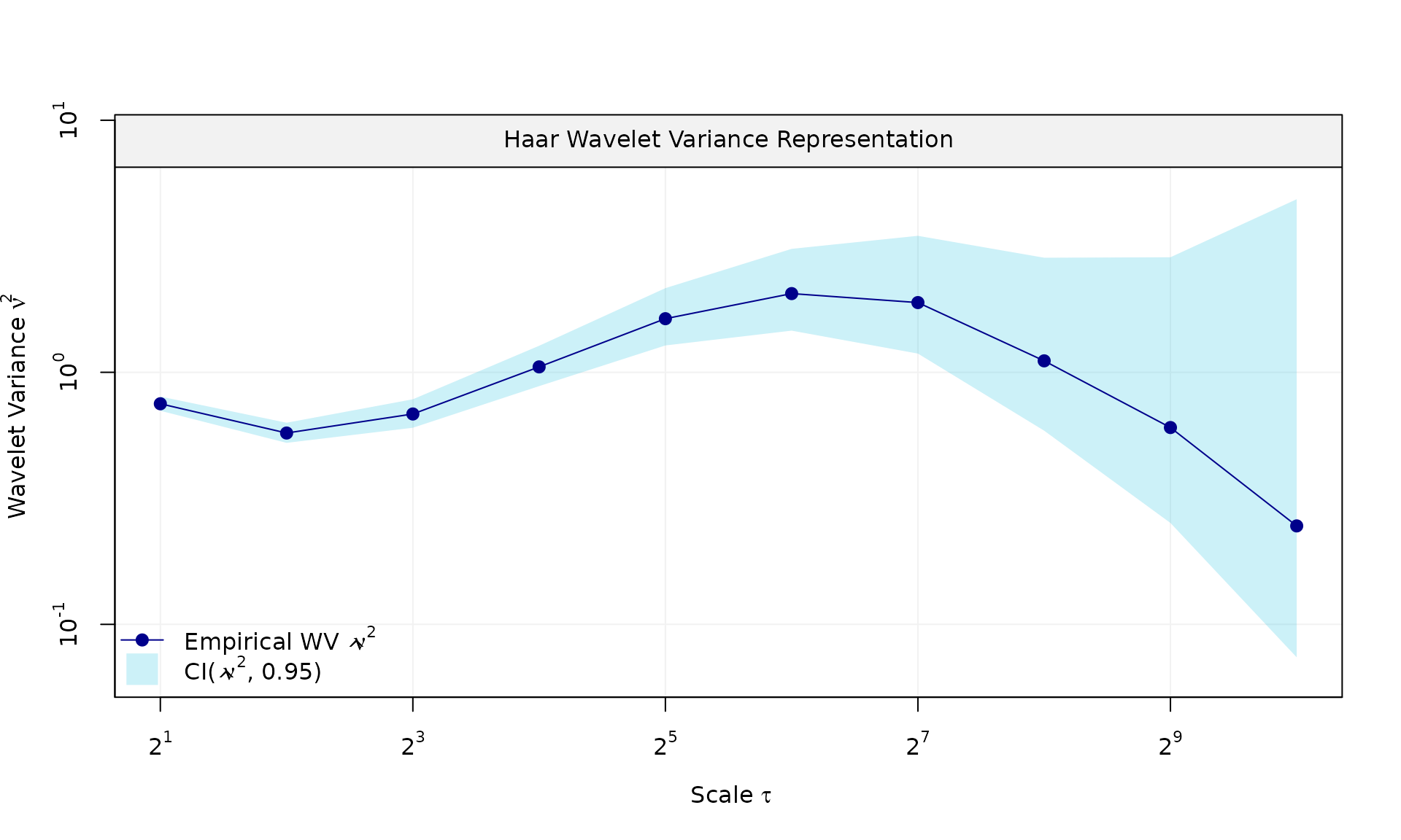
y = X %*% beta + eps

# generate missingness
mod_missing = markov_two_states(p1 = 0.05, p2 = .95)
Z = generate(mod_missing, n = n, seed = 123)
plot(Z)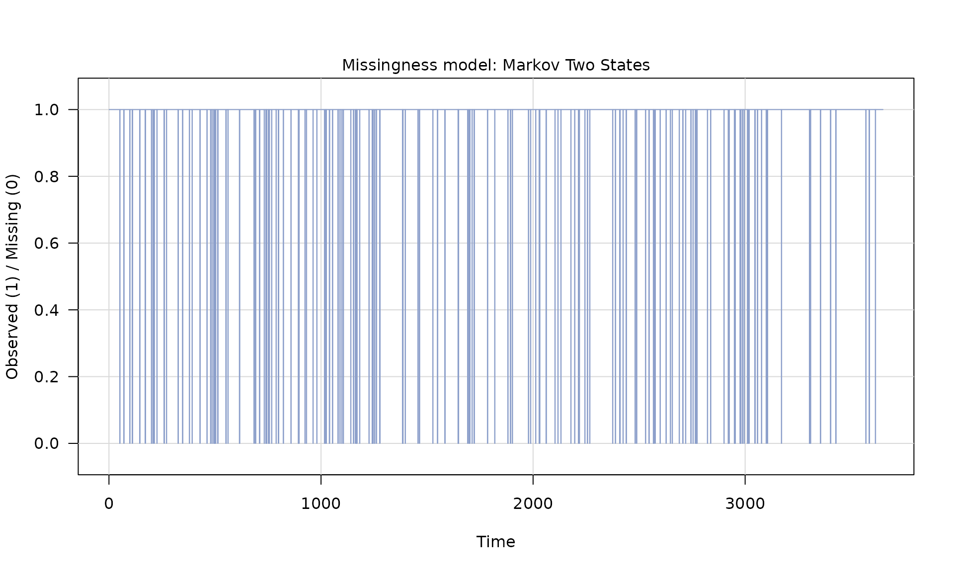
Z_process = Z$series
y_observed = ifelse(Z_process == 1, y, NA)
plot(X[, 2], y_observed, type = "l", main = "Simulated y (WN + AR1)")
# add grey boxes at missing indices (x ± eps) to visualize NA locations;
# unlike `vignettes/gmwmx2_new.Rmd`, which plots the fully observed series
na_idx <- which(is.na(y_observed))

# choose epsilon relative to x spacing
dx <- median(diff(X[, 2]), na.rm = TRUE)
eps <- 0.45 * dx

ylim <- par("usr")[3:4]
for (i in na_idx) {
  rect(
    xleft = X[i, 2] - eps,
    xright = X[i, 2] + eps,
    ybottom = ylim[1],
    ytop = ylim[2],
    col = adjustcolor("grey20", alpha.f = 0.5),
    border = NA
  )
}

lines(X[, 2], y_observed)
We then fit the dependent‑error regression using
gmwmx2_new(), which accounts for the stochastic error model
and the missing observations.
#
# Fit model (WN + AR1)

fit = gmwmx2_new(X = X, y = y_observed, model = wn() + ar1() )
print(fit)
## GMWMX fit
## Estimate Std.Error
## beta1 1.778606 0.702485
## beta2 0.009616 0.000333
## beta3 1.847444 0.467891
## beta4 0.947159 0.463950
##
## Missingness model
## Proportion missing : 0.0455
## p1 : 0.0451
## p2 : 0.9458
## p* : 0.9545
##
## Stochastic model
## Sum of 2 processes
## [1] White Noise
## Estimated parameters : sigma2 = 1.076
## [2] AR(1)
## Estimated parameters : phi = 0.9562, sigma2 = 0.8705
##
## Runtime (seconds)
## Total : 1.2656
B = 100
mat_res = matrix(NA, nrow=B, ncol=19)
for(b in seq(B)){

  eps = generate(ar1(phi=0.95, sigma2=20) + wn(20), n=n, seed = (123 + b))$series
  y = X %*% beta + eps
  Z = generate(mod_missing, n = n, seed = 123 + b)$series
  y_observed = ifelse(Z == 1, y, NA)
  fit = gmwmx2_new(X = X, y = y_observed, model = wn() + ar1() )
  # mispecified model assuming white noise as the stochastic model and only on observed data
  fit2 = lm(y_observed~X[,2] + X[,3] + X[,4])

  mat_res[b, ] = c(fit$beta_hat, fit$std_beta_hat,
                   summary(fit2)$coefficients[,1],
                   summary(fit2)$coefficients[,2],
                   fit$theta_domain$`AR(1)_2`,
                   fit$theta_domain$`White Noise_1`)
  # cat("Iteration ", b, " completed.\n")
}
We now assess inference quality under missingness by repeating the
simulation, fitting the correct dependent‑error model with
gmwmx2_new(), and comparing against a misspecified OLS fit
that treats the errors as i.i.d. and uses only observed data.
# compute empirical coverage
mat_res_df = as.data.frame(mat_res)
colnames(mat_res_df) = c("gmwmx_beta0_hat", "gmwmx_beta1_hat",
                         "gmwmx_beta2_hat", "gmwmx_beta3_hat",
                         "gmwmx_std_beta0_hat", "gmwmx_std_beta1_hat",
                         "gmwmx_std_beta2_hat", "gmwmx_std_beta3_hat",
                         "lm_beta0_hat", "lm_beta1_hat", "lm_beta2_hat", "lm_beta3_hat",
                         "lm_std_beta0_hat", "lm_std_beta1_hat", "lm_std_beta2_hat", "lm_std_beta3_hat",
                         "phi_ar1","sigma_2_ar1" ,"sigma_2_wn")


# Plot empirical distributions (beta and stochastic parameters)

par(mfrow = c(1, 4))
boxplot_mean_dot(mat_res_df[, c("gmwmx_beta0_hat")],las=1,
                 names = c("beta0"),
                 main = expression(beta[0]), ylab = "Estimate")
abline(h = beta[1], col = "black", lwd = 2)

boxplot_mean_dot(mat_res_df[, c("gmwmx_beta1_hat")],las=1,
                 names = c("beta1"),
                 main = expression(beta[1]), ylab = "Estimate")
abline(h = beta[2], col = "black", lwd = 2)

boxplot_mean_dot(mat_res_df[, c("gmwmx_beta2_hat")],las=1,
                 names = c("beta2"),
                 main = expression(beta[2]), ylab = "Estimate")
abline(h = beta[3], col = "black", lwd = 2)

boxplot_mean_dot(mat_res_df[, c("gmwmx_beta3_hat")],las=1,
                 names = c("beta3"),
                 main = expression(beta[3]), ylab = "Estimate")
abline(h = beta[4], col = "black", lwd = 2)
par(mfrow = c(1, 3))

boxplot_mean_dot(mat_res_df$phi_ar1,las=1,
                 names = c("phi_ar1"),
                 main = expression(phi["AR1"]), ylab = "Estimate")
abline(h = phi_ar1, col = "black", lwd = 2)

boxplot_mean_dot(mat_res_df$sigma_2_ar1,las=1,
                 names = c("phi_ar1"),
                 main = expression(sigma["AR1"]^2), ylab = "Estimate")
abline(h = sigma2_ar1, col = "black", lwd = 2)

boxplot_mean_dot(mat_res_df$sigma_2_wn,las=1,
                 names = c("phi_ar1"),
                 main = expression(sigma["WN"]^2), ylab = "Estimate")
abline(h = sigma2_wn, col = "black", lwd = 2)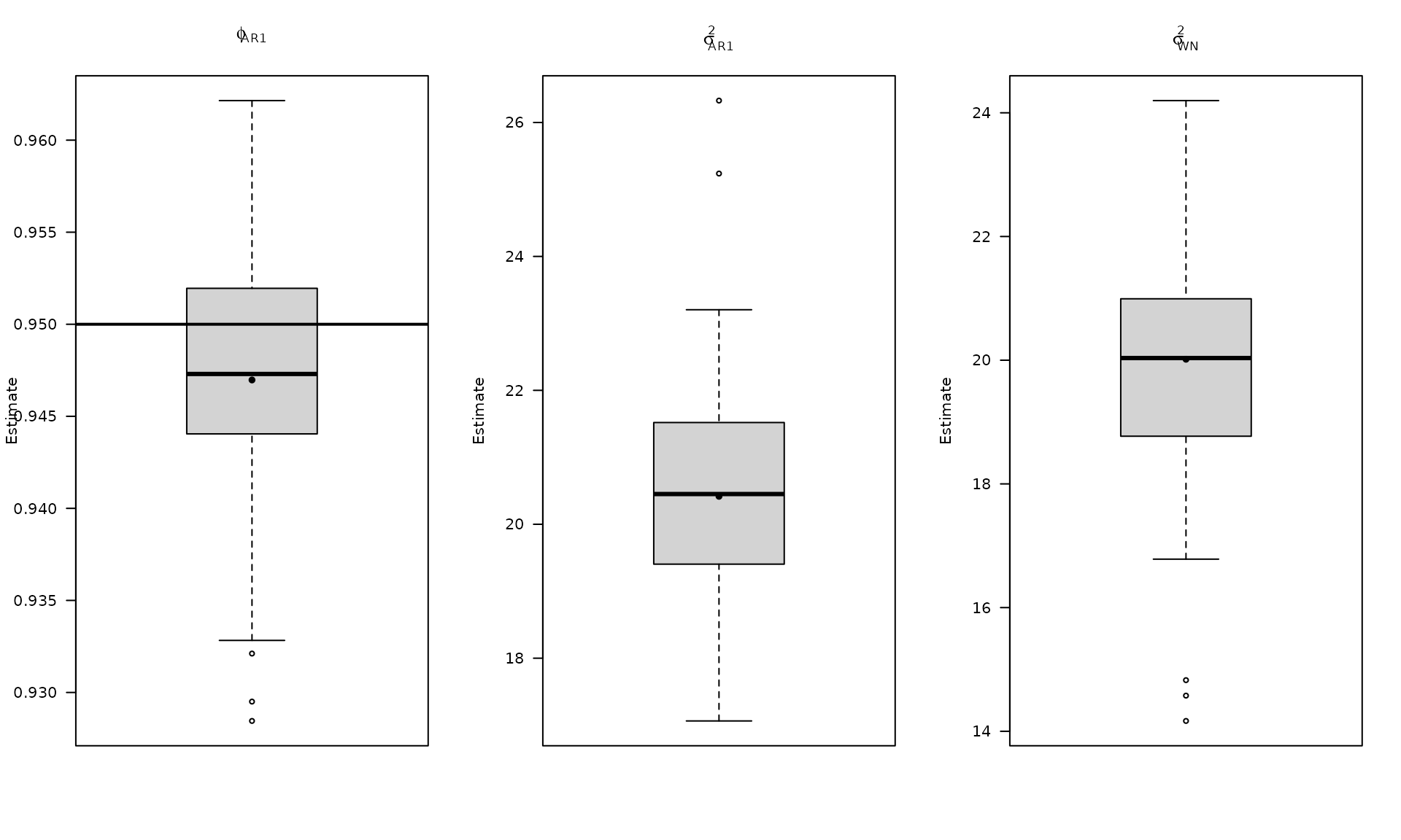
The boxplots summarize the empirical distribution of the regression estimates and stochastic parameters across Monte Carlo replications, with the true values shown as horizontal lines.
We report the empirical fraction of times the true
entries fall inside the estimated intervals for both
gmwmx2_new() and OLS.
# Compute empirical coverage of confidence intervals for beta

zval = qnorm(0.975)
mat_res_df$upper_ci_gmwmx_beta0 = mat_res_df$gmwmx_beta0_hat + zval * mat_res_df$gmwmx_std_beta0_hat
mat_res_df$lower_ci_gmwmx_beta0 = mat_res_df$gmwmx_beta0_hat - zval * mat_res_df$gmwmx_std_beta0_hat
mat_res_df$upper_ci_gmwmx_beta1 = mat_res_df$gmwmx_beta1_hat + zval * mat_res_df$gmwmx_std_beta1_hat
mat_res_df$lower_ci_gmwmx_beta1 = mat_res_df$gmwmx_beta1_hat - zval * mat_res_df$gmwmx_std_beta1_hat
# empirical coverage of gmwmx beta
dplyr::between(rep(beta[1], B), mat_res_df$lower_ci_gmwmx_beta0, mat_res_df$upper_ci_gmwmx_beta0) %>% mean()
## [1] 0.94
dplyr::between(rep(beta[2], B), mat_res_df$lower_ci_gmwmx_beta1, mat_res_df$upper_ci_gmwmx_beta1) %>% mean()## [1] 0.91
# do the same for lm beta
mat_res_df$upper_ci_lm_beta0 = mat_res_df$lm_beta0_hat + zval * mat_res_df$lm_std_beta0_hat
mat_res_df$lower_ci_lm_beta0 = mat_res_df$lm_beta0_hat - zval * mat_res_df$lm_std_beta0_hat
mat_res_df$upper_ci_lm_beta1 = mat_res_df$lm_beta1_hat + zval * mat_res_df$lm_std_beta1_hat
mat_res_df$lower_ci_lm_beta1 = mat_res_df$lm_beta1_hat - zval * mat_res_df$lm_std_beta1_hat
dplyr::between(rep(beta[1], B), mat_res_df$lower_ci_lm_beta0, mat_res_df$upper_ci_lm_beta0) %>% mean()
## [1] 0.21
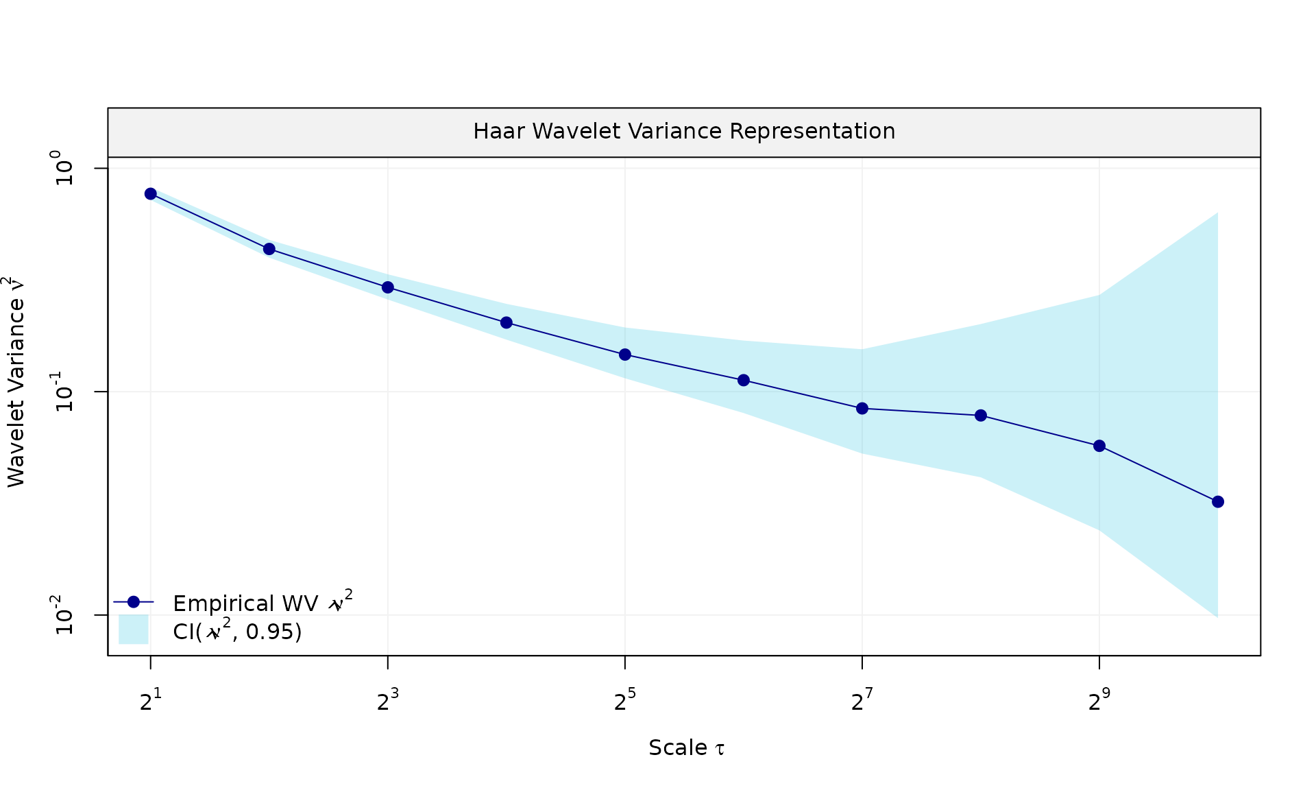
dplyr::between(rep(beta[2], B), mat_res_df$lower_ci_lm_beta1, mat_res_df$upper_ci_lm_beta1) %>% mean()## [1] 0.25We now repeat the workflow for a long‑memory error model (white noise
+ stationary power‑law). The steps mirror the AR(1) case: simulate with
missingness, fit gmwmx2_new(), and compare to a
misspecified OLS fit.
The parameter controls the long‑memory behavior of the power‑law component.
# Example 2: White noise + stationary power-law


kappa_pl <- -0.8
sigma2_wn <- 1
sigma2_pl <- .8
eps_pl = generate(wn(sigma2_wn) + pl(kappa = kappa_pl, sigma2 = sigma2_pl),
                  n = n, seed = 1234)
plot(eps_pl$series, type = "l")
Z_process = Z$series
y_observed = ifelse(Z_process == 1, y_pl, NA)


fit_pl = gmwmx2_new(X = X, y = y_observed, model = wn() + pl())
fit_pl
## GMWMX fit
## Estimate Std.Error
## beta1 0.86562 0.5214672
## beta2 0.01028 0.0001791
## beta3 2.19066 0.1051664
## beta4 1.51667 0.1029350
##
## Missingness model
## Proportion missing : 0.0485
## p1 : 0.0475
## p2 : 0.9322
## p* : 0.9515
##
## Stochastic model
## Sum of 2 processes
## [1] White Noise
## Estimated parameters : sigma2 = 0.8601
## [2] Stationary PowerLaw
## Estimated parameters : kappa = -0.7344, sigma2 = 0.9371
##
## Runtime (seconds)
## Total : 0.5931As before, we keep the same missingness mechanism so that differences are driven by the error model rather than by the observation pattern.
Monte Carlo replication for the power‑law case.
B_pl = 100
mat_res_pl = matrix(NA, nrow = B_pl, ncol = 19)
for(b in seq(B_pl)){
  eps = generate(wn(sigma2_wn) + pl(kappa = kappa_pl, sigma2 = sigma2_pl),
                 n = n, seed = (123 + b))$series
  y = X %*% beta + eps

  Z = generate(mod_missing, n = n, seed = (123 + b))
  Z_process = Z$series
  y_observed = ifelse(Z_process == 1, y, NA)

  fit = gmwmx2_new(X = X, y = y_observed, model = wn() + pl())
  fit2 = lm(y_observed~X[,2] + X[,3] + X[,4])

  mat_res_pl[b, ] = c(fit$beta_hat, fit$std_beta_hat,
                      summary(fit2)$coefficients[,1],
                      summary(fit2)$coefficients[,2],
                      fit$theta_domain$`Stationary PowerLaw_2`,
                      fit$theta_domain$`White Noise_1`)
  # cat("Iteration ", b, " \n")
}
Aggregate the Monte Carlo results and visualize regression estimates.
The next plots focus on the distribution of estimates under the power‑law error model.
mat_res_pl_df = as.data.frame(mat_res_pl)
colnames(mat_res_pl_df) = c("gmwmx_beta0_hat", "gmwmx_beta1_hat",
                            "gmwmx_beta2_hat", "gmwmx_beta3_hat",
                            "gmwmx_std_beta0_hat", "gmwmx_std_beta1_hat",
                            "gmwmx_std_beta2_hat", "gmwmx_std_beta3_hat",
                            "lm_beta0_hat", "lm_beta1_hat", "lm_beta2_hat", "lm_beta3_hat",
                            "lm_std_beta0_hat", "lm_std_beta1_hat",
                            "lm_std_beta2_hat", "lm_std_beta3_hat",
                            "kappa_pl","sigma2_pl" ,"sigma2_wn")


# Plot empirical distributions (beta and stochastic parameters)


par(mfrow = c(1, 4))
boxplot_mean_dot(mat_res_df[, c("gmwmx_beta0_hat")],las=1,
                 names = c("beta0"),
                 main = expression(beta[0]), ylab = "Estimate")
abline(h = beta[1], col = "black", lwd = 2)

boxplot_mean_dot(mat_res_df[, c("gmwmx_beta1_hat")],las=1,
                 names = c("beta1"),
                 main = expression(beta[1]), ylab = "Estimate")
abline(h = beta[2], col = "black", lwd = 2)

boxplot_mean_dot(mat_res_df[, c("gmwmx_beta2_hat")],las=1,
                 names = c("beta2"),
                 main = expression(beta[2]), ylab = "Estimate")
abline(h = beta[3], col = "black", lwd = 2)

boxplot_mean_dot(mat_res_df[, c("gmwmx_beta3_hat")],las=1,
                 names = c("beta3"),
                 main = expression(beta[3]), ylab = "Estimate")
abline(h = beta[4], col = "black", lwd = 2)
Plot the estimated stochastic parameter estimates for the power‑law model.
par(mfrow = c(1, 3))

boxplot_mean_dot(mat_res_pl_df$kappa_pl,las=1,
                 main = expression(kappa["PL"]), ylab = "Estimate")
abline(h = kappa_pl, col = "black", lwd = 2)

boxplot_mean_dot(mat_res_pl_df$sigma2_pl,las=1,
                 main = expression(sigma["PL"]^2), ylab = "Estimate")
abline(h = sigma2_pl, col = "black", lwd = 2)

boxplot_mean_dot(mat_res_pl_df$sigma2_wn,las=1,
                 names = c("phi_ar1"),
                 main = expression(sigma["WN"]^2), ylab = "Estimate")
abline(h = sigma2_wn, col = "black", lwd = 2)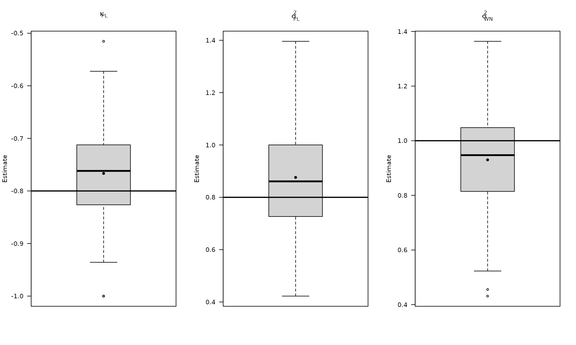
Compute empirical coverage for the regression coefficients under the power‑law error model and compare against OLS.
# Compute empirical coverage of confidence intervals for beta

zval = qnorm(0.975)
mat_res_pl_df$upper_ci_gmwmx_beta0 = mat_res_pl_df$gmwmx_beta0_hat + zval * mat_res_pl_df$gmwmx_std_beta0_hat
mat_res_pl_df$lower_ci_gmwmx_beta0 = mat_res_pl_df$gmwmx_beta0_hat - zval * mat_res_pl_df$gmwmx_std_beta0_hat
mat_res_pl_df$upper_ci_gmwmx_beta1 = mat_res_pl_df$gmwmx_beta1_hat + zval * mat_res_pl_df$gmwmx_std_beta1_hat
mat_res_pl_df$lower_ci_gmwmx_beta1 = mat_res_pl_df$gmwmx_beta1_hat - zval * mat_res_pl_df$gmwmx_std_beta1_hat
# empirical coverage of gmwmx beta
dplyr::between(rep(beta[1], B_pl), mat_res_pl_df$lower_ci_gmwmx_beta0, mat_res_pl_df$upper_ci_gmwmx_beta0) %>% mean()
## [1] 0.82
dplyr::between(rep(beta[2], B_pl), mat_res_pl_df$lower_ci_gmwmx_beta1, mat_res_pl_df$upper_ci_gmwmx_beta1) %>% mean()## [1] 0.89
# do the same for lm beta
mat_res_pl_df$upper_ci_lm_beta0 = mat_res_pl_df$lm_beta0_hat + zval * mat_res_pl_df$lm_std_beta0_hat
mat_res_pl_df$lower_ci_lm_beta0 = mat_res_pl_df$lm_beta0_hat - zval * mat_res_pl_df$lm_std_beta0_hat
mat_res_pl_df$upper_ci_lm_beta1 = mat_res_pl_df$lm_beta1_hat + zval * mat_res_pl_df$lm_std_beta1_hat
mat_res_pl_df$lower_ci_lm_beta1 = mat_res_pl_df$lm_beta1_hat - zval * mat_res_pl_df$lm_std_beta1_hat
dplyr::between(rep(beta[1], B_pl), mat_res_pl_df$lower_ci_lm_beta0, mat_res_pl_df$upper_ci_lm_beta0) %>% mean()
## [1] 0.08
dplyr::between(rep(beta[2], B_pl), mat_res_pl_df$lower_ci_lm_beta1, mat_res_pl_df$upper_ci_lm_beta1) %>% mean()## [1] 0.15Finally, we repeat the missing‑data inference workflow for a flicker‑noise error model.
# Example 3: White noise + flicker


sigma2_wn_fl <- 1
sigma2_fl <- 1
eps_fl = generate(wn(sigma2_wn_fl) + flicker(sigma2 = sigma2_fl),
                  n = n, seed = 123)
plot(eps_fl$series, type = "l")

y_fl = X %*% beta + eps_fl$series
Z = generate(mod_missing, n = n, seed = 1234)
plot(Z)
Z_process = Z$series
y_observed = ifelse(Z_process == 1, y_fl, NA)
fit_fl = gmwmx2_new(X = X, y = y_observed, model = wn() + flicker())
fit_fl## GMWMX fit
## Estimate Std.Error
## beta1 0.44556 0.8698443
## beta2 0.01013 0.0004128
## beta3 1.95655 0.1746552
## beta4 1.53098 0.1689793
##
## Missingness model
## Proportion missing : 0.0485
## p1 : 0.0475
## p2 : 0.9322
## p* : 0.9515
##
## Stochastic model
## Sum of 2 processes
## [1] White Noise
## Estimated parameters : sigma2 = 1.092
## [2] Flicker
## Estimated parameters : sigma2 = 0.8848
##
## Runtime (seconds)
## Total : 1.2116Monte Carlo replication for the flicker‑noise case.
B_fl = 100
mat_res_fl = matrix(NA, nrow = B_fl, ncol = 18)
for(b in seq(B_fl)){
  eps = generate(wn(sigma2_wn_fl) + flicker(sigma2 = sigma2_fl),
                 n = n, seed = (123 + b))$series
  y = X %*% beta + eps


  Z = generate(mod_missing, n = n, seed = (123 + b))
  Z_process = Z$series
  y_observed = ifelse(Z_process == 1, y, NA)


  fit = gmwmx2_new(X = X, y = y_observed, model = wn() + flicker())
  fit2 = lm(y_observed~X[,2] + X[,3] + X[,4])

  mat_res_fl[b, ] = c(fit$beta_hat, fit$std_beta_hat,
                      summary(fit2)$coefficients[,1],
                      summary(fit2)$coefficients[,2],
                      fit$theta_domain$`Flicker_2`,
                      fit$theta_domain$`White Noise_1`)
  # cat("Iteration ", b, " \n")
}
mat_res_fl_df = as.data.frame(mat_res_fl)
colnames(mat_res_fl_df) = c("gmwmx_beta0_hat", "gmwmx_beta1_hat",
                            "gmwmx_beta2_hat", "gmwmx_beta3_hat",
                            "gmwmx_std_beta0_hat", "gmwmx_std_beta1_hat",
                            "gmwmx_std_beta2_hat", "gmwmx_std_beta3_hat",
                            "lm_beta0_hat", "lm_beta1_hat", "lm_beta2_hat", "lm_beta3_hat",
                            "lm_std_beta0_hat", "lm_std_beta1_hat",
                            "lm_std_beta2_hat", "lm_std_beta3_hat",
                            "sigma2_fl" ,"sigma2_wn")
Compute empirical coverage for the flicker‑noise case.
# Compute empirical coverage of confidence intervals for beta

zval = qnorm(0.975)
mat_res_fl_df$upper_ci_gmwmx_beta0 = mat_res_fl_df$gmwmx_beta0_hat + zval * mat_res_fl_df$gmwmx_std_beta0_hat
mat_res_fl_df$lower_ci_gmwmx_beta0 = mat_res_fl_df$gmwmx_beta0_hat - zval * mat_res_fl_df$gmwmx_std_beta0_hat
mat_res_fl_df$upper_ci_gmwmx_beta1 = mat_res_fl_df$gmwmx_beta1_hat + zval * mat_res_fl_df$gmwmx_std_beta1_hat
mat_res_fl_df$lower_ci_gmwmx_beta1 = mat_res_fl_df$gmwmx_beta1_hat - zval * mat_res_fl_df$gmwmx_std_beta1_hat
# empirical coverage of gmwmx beta
dplyr::between(rep(beta[1], B_fl), mat_res_fl_df$lower_ci_gmwmx_beta0, mat_res_fl_df$upper_ci_gmwmx_beta0) %>% mean()
## [1] 0.97
dplyr::between(rep(beta[2], B_fl), mat_res_fl_df$lower_ci_gmwmx_beta1, mat_res_fl_df$upper_ci_gmwmx_beta1) %>% mean()## [1] 0.93
# do the same for lm beta
mat_res_fl_df$upper_ci_lm_beta0 = mat_res_fl_df$lm_beta0_hat + zval * mat_res_fl_df$lm_std_beta0_hat
mat_res_fl_df$lower_ci_lm_beta0 = mat_res_fl_df$lm_beta0_hat - zval * mat_res_fl_df$lm_std_beta0_hat
mat_res_fl_df$upper_ci_lm_beta1 = mat_res_fl_df$lm_beta1_hat + zval * mat_res_fl_df$lm_std_beta1_hat
mat_res_fl_df$lower_ci_lm_beta1 = mat_res_fl_df$lm_beta1_hat - zval * mat_res_fl_df$lm_std_beta1_hat
dplyr::between(rep(beta[1], B_fl), mat_res_fl_df$lower_ci_lm_beta0, mat_res_fl_df$upper_ci_lm_beta0) %>% mean()
## [1] 0.08
dplyr::between(rep(beta[2], B_fl), mat_res_fl_df$lower_ci_lm_beta1, mat_res_fl_df$upper_ci_lm_beta1) %>% mean()## [1] 0.07
# Plot empirical distributions (beta and stochastic parameters)Plot regression estimates for the flicker‑noise case.
par(mfrow = c(1, 4))
boxplot_mean_dot(mat_res_df[, c("gmwmx_beta0_hat")],las=1,
                 names = c("beta0"),
                 main = expression(beta[0]), ylab = "Estimate")
abline(h = beta[1], col = "black", lwd = 2)

boxplot_mean_dot(mat_res_df[, c("gmwmx_beta1_hat")],las=1,
                 names = c("beta1"),
                 main = expression(beta[1]), ylab = "Estimate")
abline(h = beta[2], col = "black", lwd = 2)

boxplot_mean_dot(mat_res_df[, c("gmwmx_beta2_hat")],las=1,
                 names = c("beta2"),
                 main = expression(beta[2]), ylab = "Estimate")
abline(h = beta[3], col = "black", lwd = 2)

boxplot_mean_dot(mat_res_df[, c("gmwmx_beta3_hat")],las=1,
                 names = c("beta3"),
                 main = expression(beta[3]), ylab = "Estimate")
abline(h = beta[4], col = "black", lwd = 2)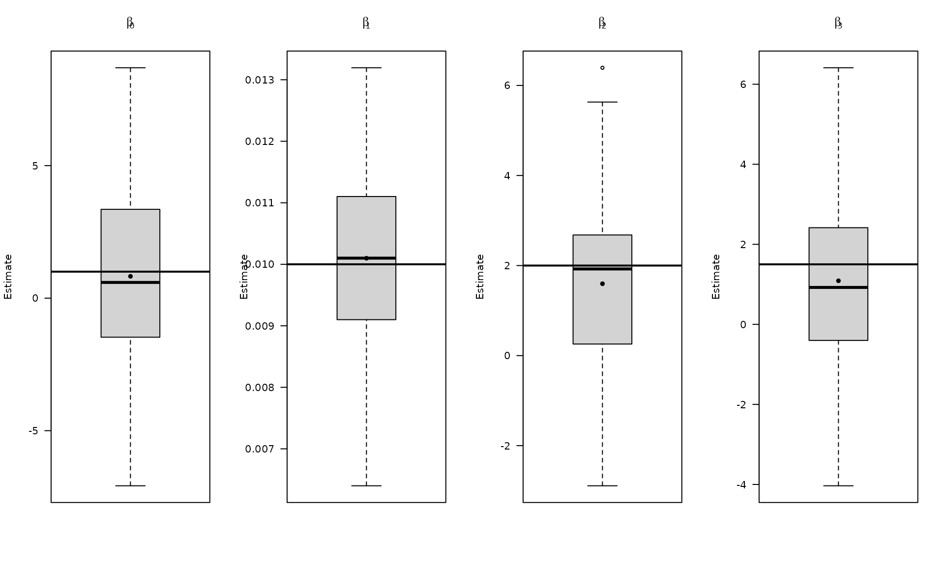
Plot stochastic parameter estimates for the flicker‑noise case.
par(mfrow = c(1, 2))

boxplot_mean_dot(mat_res_fl_df$sigma2_fl,las=1,
                 main = expression(sigma["FL"]^2), ylab = "Estimate")
abline(h = sigma2_fl, col = "black", lwd = 2)

boxplot_mean_dot(mat_res_fl_df$sigma2_wn,las=1,
                 names = c("phi_ar1"),
                 main = expression(sigma["WN"]^2), ylab = "Estimate")
abline(h = sigma2_wn_fl, col = "black", lwd = 2)