simts Vignettes

Time Series Simulation

In this section, we briefly list, describe, and provide the syntax used to simulate time series data using the simts package. The following list includes some basic models available in this package:

• White Noise WN()
• Quantization Noise QN()
• Random Walk RW()
• Drift DR()
• First-order Autoregressive AR1()
• Autoregressive AR()
• First-order Moving Average MA1()
• Moving Average Process MA()
• Gauss-Markov GM()
• Autoregressive Moving Average ARMA()
• Integrated Autoregressive Moving Average ARIMA()
• Seasonal Autoregressive Integrated Moving Average SARIMA()
• Seasonal Autoregressive Moving Average SARMA()
• Sinusoidal Process SIN()
• Quantization Noise QN()
• Fractional Gaussian Noise FGN()
• Power Law Process PLP()
• Matèrn Process MAT()

Quantization noise is a less known process that is used in engineering applications. It can be described in layperson terms as being a good estimator of a rounding error.

The code below shows how to call the function gen_gts(), which allows the user to generate samples from the above model specifications.

# Set seed for reproducibility
set.seed(1337)

# Number of observations
n = 10^4

# Generate a White Noise Process
wn = gen_gts(n, WN(sigma2 = 1)) 

# Generate a Quantization Noise
qn = gen_gts(n, QN(q2 = .5)) 

# Generate a Random Walk
rw = gen_gts(n, RW(gamma2 = .75)) 

By applying the plot() function on the result of a gen_gts() simulation, we can observe a visualization of our simulated data.

par(mfrow = c(3,1))
plot(wn)
plot(qn)
plot(rw)

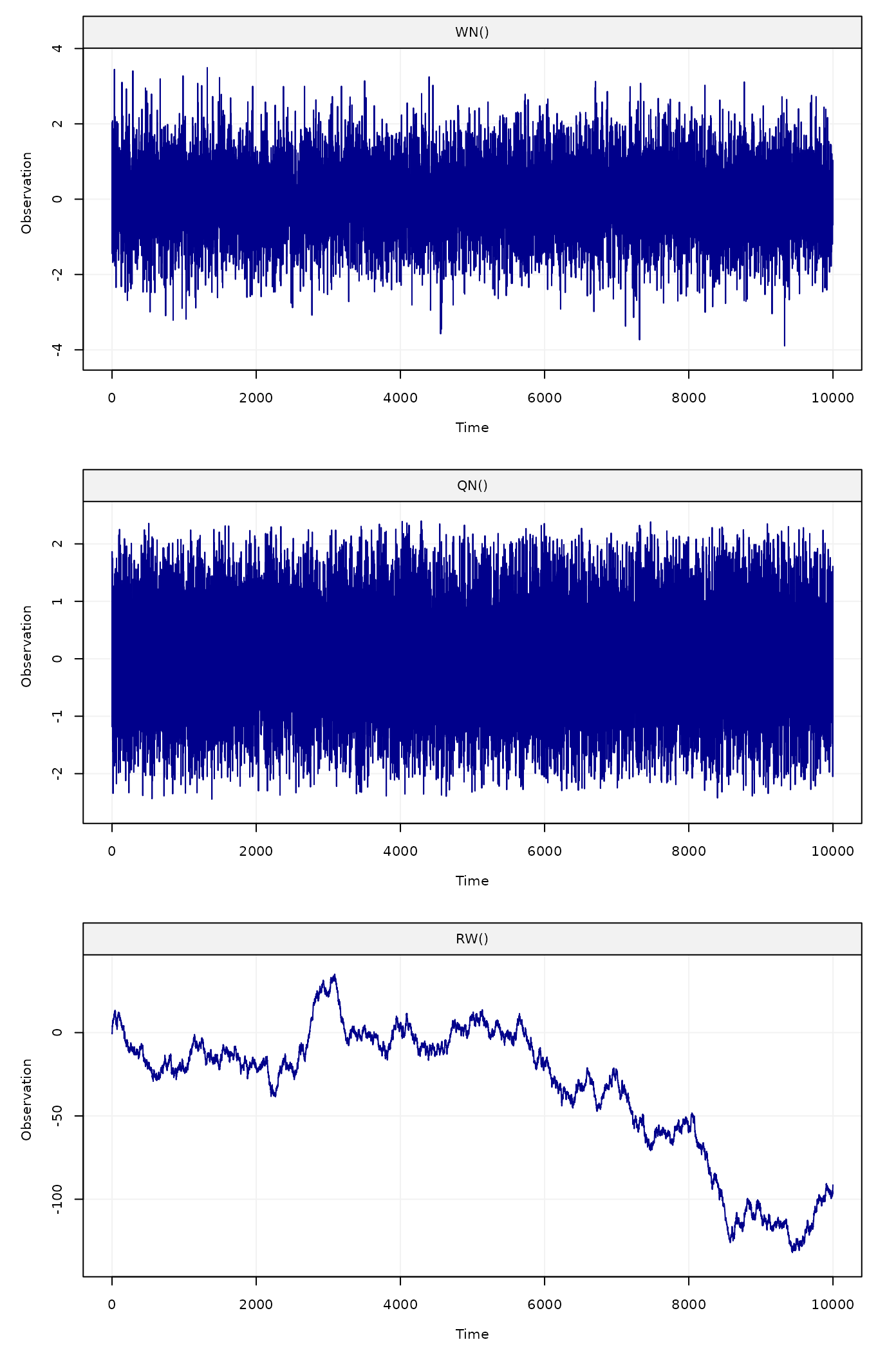
Figure 1: Simulated white noise process (top panel), quantiation noise (middle panel) and random walk process (bottom panel)

Another example with a SARIMA model is given below:

# Generate an SARIMA(1,0,1)x(2,1,1)[12]
sarima = gen_gts(n, SARIMA(ar = 0.3, i = 0, ma = -0.27,
                        sar = c(-0.12, -0.2), si = 1, sma = -0.9,
                        sigma2 = 1.5, s = 12))
# Plot simulation of SARIMA(1,0,1)x(2,1,1)[12]
plot(sarima)

Figure 2: Simulated SARIMA(1,0,1)x(2,1,1)[12] process

The simts package therefore allows users to easily simulate from a wide variety of classical time series models, but does not limit itself to these models. Indeed, under some restrictions, these models can be combined in different ways to deliver many state-space (latent) models which can be represented as the sum of basic models.

simts’s user friendly interface allows for easy construction of such linear state-space models. In fact, to specify that a certain model is a combination of different models, all that is needed is the “+” symbol between them. For example, consider the following state-space model:

\[\begin{aligned} X_t &= X_{t-1} + \omega + U_t, \;\;\;\;\; U_t \sim \mathcal{N}(0,\gamma^2),\\ Y_t &= X_t + Z_t , \;\;\;\;\; Z_t \sim \mathcal{N}(0,\sigma^2), \end{aligned}\]

it is easy to see that this model is exactly equivalent to the sum of a random walk (with inivation variance \(\gamma^2\)), a linear drift (with slope \(\omega\)) and a white noise process (with variance \(\sigma^2\)). Therefore, it can easily be simulated as follows:

set.seed(1)
model = RW(gamma2 = 0.01) + DR(omega = 0.001) + WN(sigma2 = 1)
Yt = gen_gts(model, n = 10^3)
plot(Yt)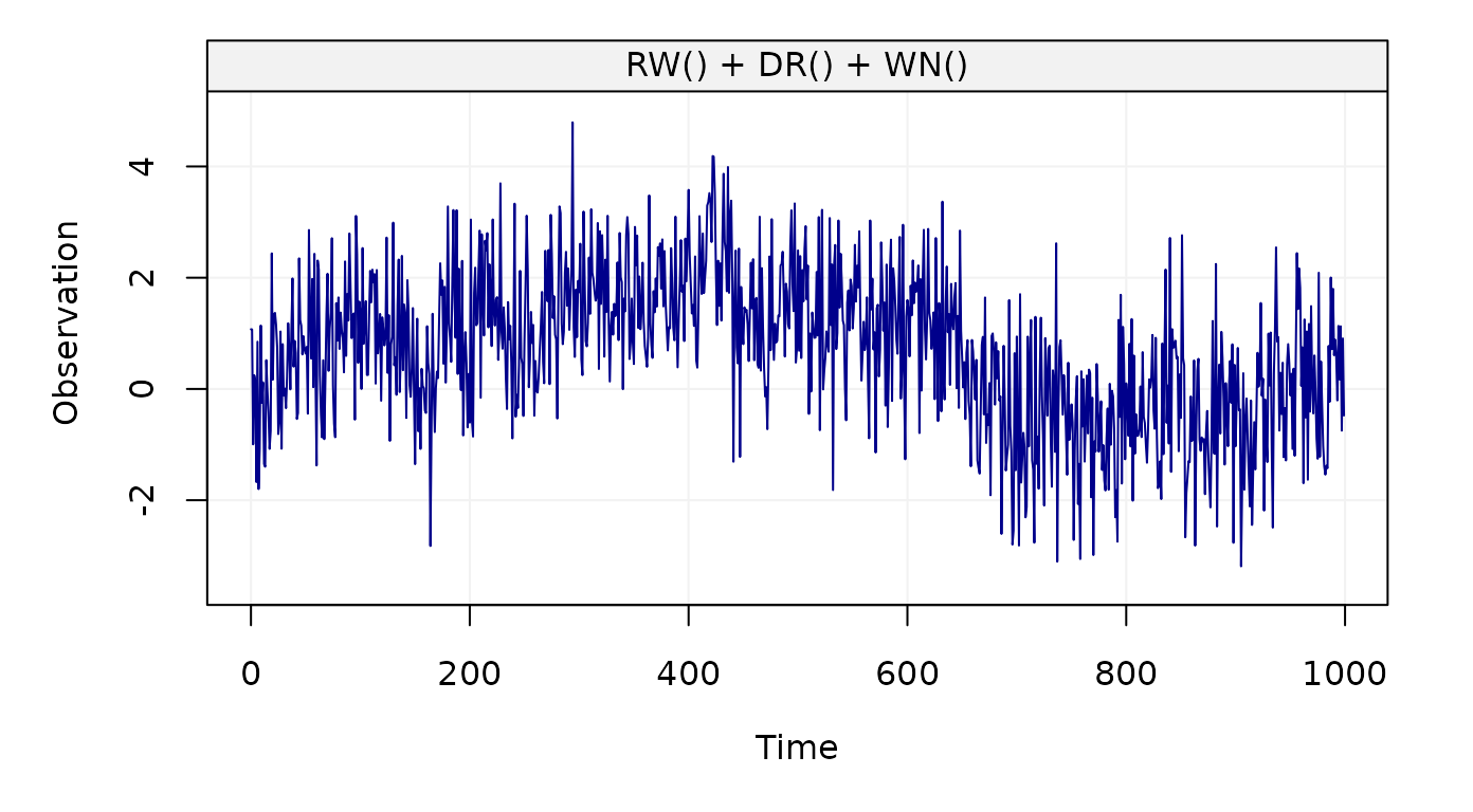

Figure 3: Simulated state-space model (RW + WN + DR)

It is also possible to retrieve and visualize the three latent used to construct such state-space model using the function gen_lts() instead of gen_gts(), as follows:

set.seed(1)
model = RW(gamma2 = 0.01) + DR(omega = 0.001) + WN(sigma2 = 1)
Yt = gen_lts(model, n = 10^3)
plot(Yt)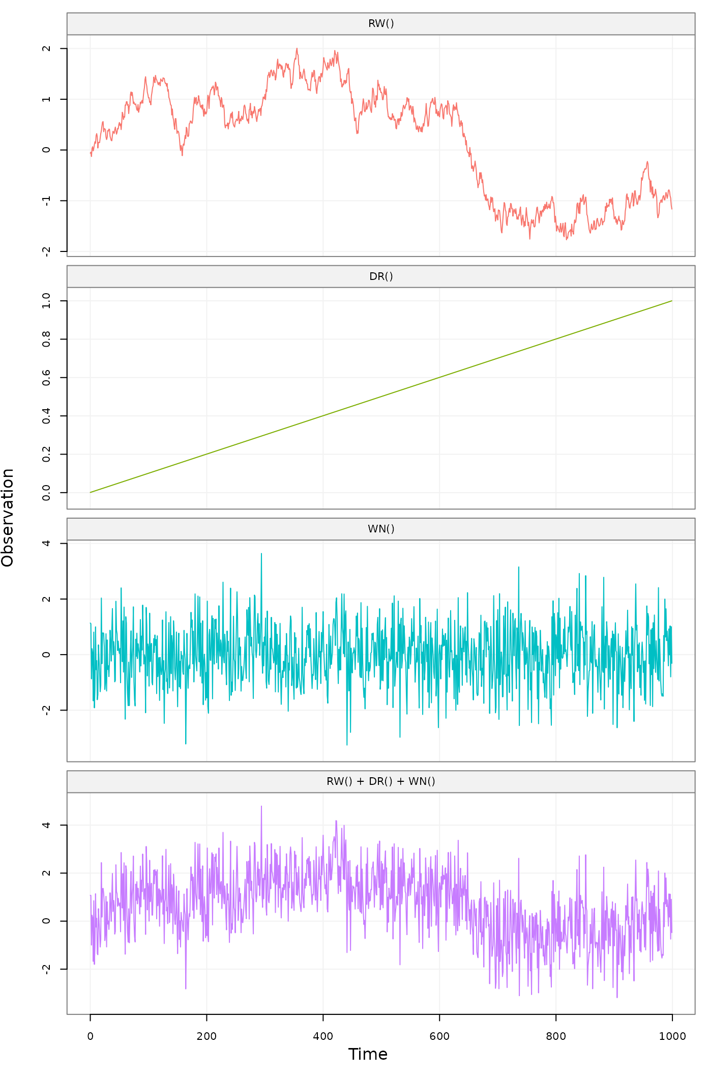

Figure 4: Simulated state-space model (RW + WN + DR) showing latent processes

Consider another example, let us suppose that different AR(1) processes are present in a state-space model. The syntax to insert “k” of these models into the state-space model is k*AR1(). So, for example, the sum of three AR1 models, a random walk and a white noise process can be given by a simple expression: 3*AR1()+RW()+WN().

Examples of simulating such models are generated below.

# Generate a ARMA(2,1) + WN()  
arma_wn_model =
  ARMA(ar = c(0.9, -0.5), ma = 0.3, sigma2 = 1) + 
  WN(sigma = 4)
arma_wn_sim = gen_gts(n = n, model  = arma_wn_model)

# Plot simulation of ARMA(2,1) + WN()
plot(arma_wn_sim)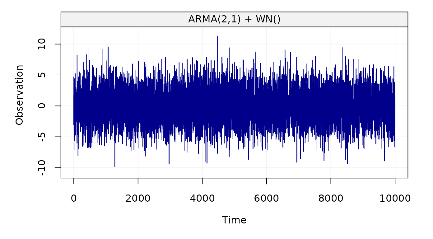

Figure 5: Simulated ARMA(2,1) + WN() process

As mentioned earlier, simts provides a function specifically designed to generate and represent latent time series models: gen_lts(). This provides users the option to visualize a breakdown of the underlying processes by applying the plot() function on the result of gen_lts().

# Generate a SARMA() + WN() 
sarma_wn_model = 
  SARMA(ar = 0, ma = 0, sar = 0.98, sma = 0, s = 10, sigma2 = 1) + 
  WN(sigma2 = 1)
sarma_wn_sim = gen_lts(n = 10^3, model = sarma_wn_model)

# Plot simulation of SARMA() + WN() 
plot(sarma_wn_sim)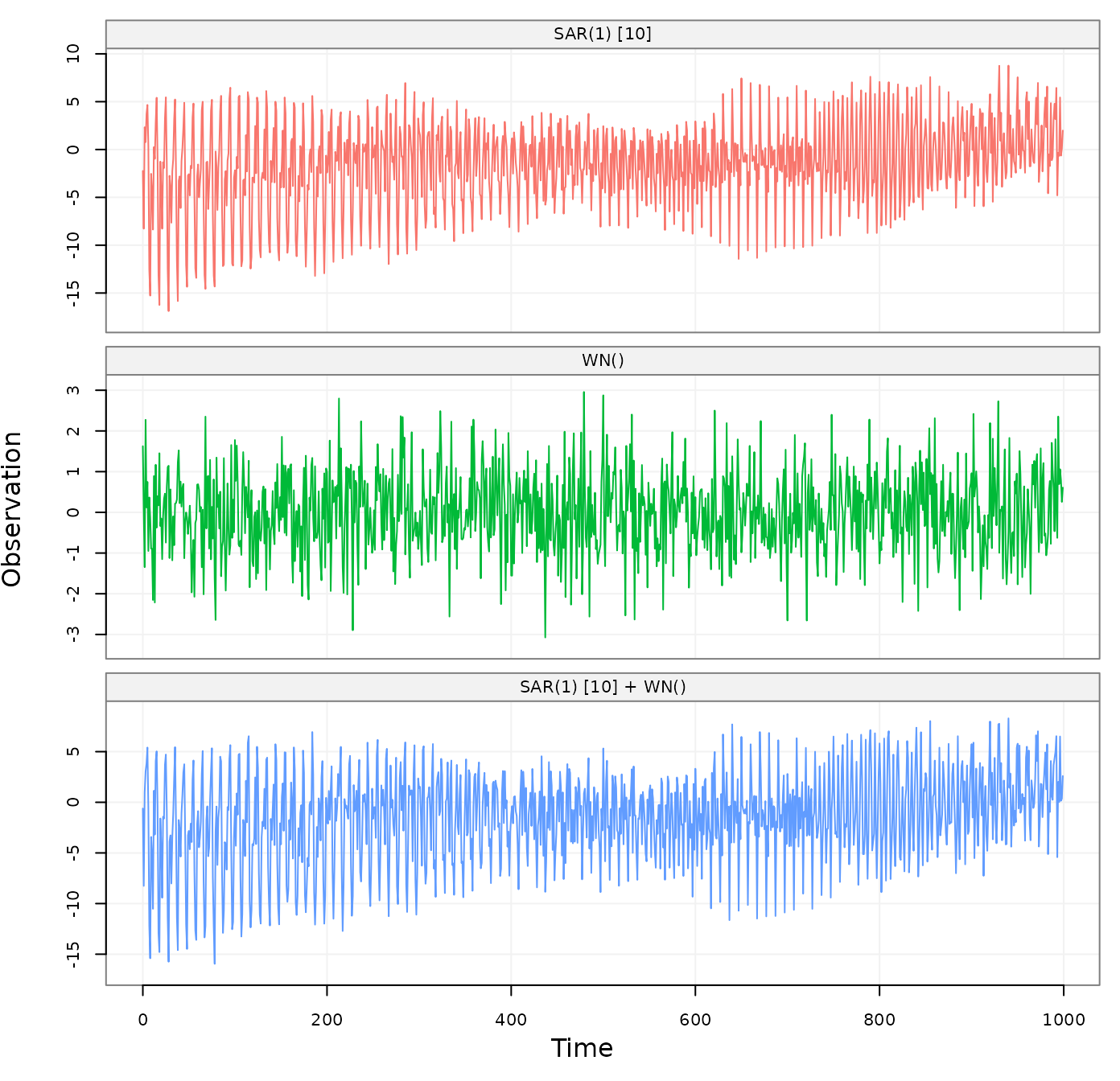

Figure 6: Simulated SARMA(1,0) x (0,1) + WN(2) process with a breakdown of the underlying latent processes

To better visualize the contribution to each process by using the sam range on the “y-axis”. This can be done with the option fixed_range = TRUE as follows:

plot(sarma_wn_sim, fixed_range = TRUE)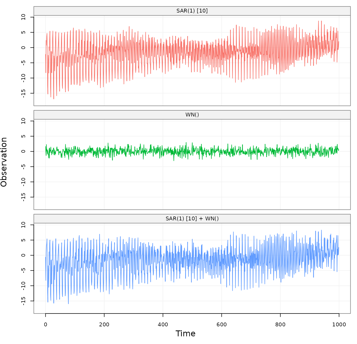

Figure 7: Simulated SARMA(1,0) x (0,1) + WN(2) process with a breakdown of the underlying latent processes

Time Series Analysis Tools

In this section, we will briefly show some of the simts package functionalities that can be applied to basic time series analysis. These functionalities are illustrated through example on the following four datasets (stored in simts):

• hydro: This time series contains the monthly precipitation from 1907 and going to 1972 for total of 781 observations taken from Hipel and McLeod (1994).
• savingrt: This dataset contains the US personal saving (after removing seasonal trends) which represent the percentage of income saved from the disposable personal income. This time series with frequency 12 starting in year 1959 and going to 2016 for a total of 691 observations.
• Nile: This time series contains the measurements of the annual flow of the river Nile at Aswan (formerly Assuan), 1871–1970, in \(10^8 m^3\) taken from Table 1 of Cobb (1978).

The code below shows how to setup a time series as a gts() object. Here, we take samples from each dataset at a rate of freq ticks per sample. By applying plot() on the result of a gts() object, we can observe a simple visualization of our data.

Hydrology dataset

Frist, we consider the hydro dataset. The code below shows how to construct a gts object and plot the resulting time series.

# Load hydro dataset
data("hydro")

# Simulate based on data
hydro = gts(as.vector(hydro), start = 1907, freq = 12, unit_ts = "in.", 
            unit_time = "year", name_ts = "Precipitation", 
            data_name = "Precipitation data from Hipel et al., (1994)")

# Plot hydro simulation
plot(hydro)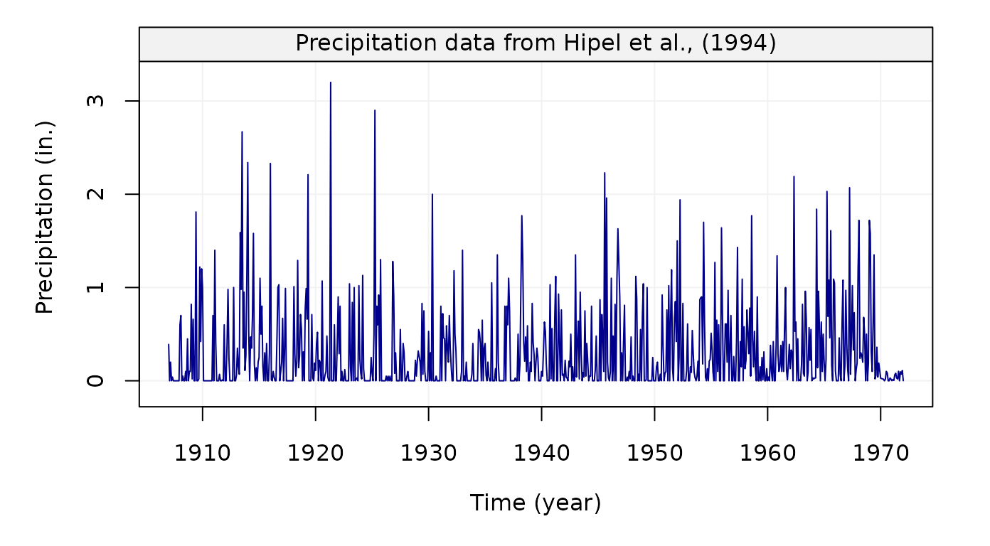

Figure 1: Monthly precipitation series from 1907 to 1972 taken from Hipel and McLeod (1994)

Using the object we created we can now compute its autocorrelation function using the auto_corr() function as follows:

# Compare the standard and robust ACF
compare_acf(hydro)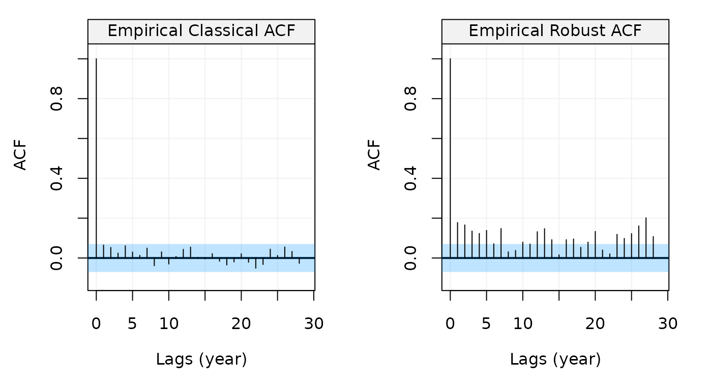

Figure 2: Standard and Robust Empirical autocorrelation functions of monthly precipitation series from Hipel and McLeod (1994)

This plot shows that no apparent autocorrelation exists when using the standard estimator of the ACF (left) but the picture changes compeltely when using the robust estimator (right). There therefore appears to be some possible contamination in the data and, if we wanted to estimate a model for the data, we would probably opt for a robust estimator. For this we can use the RGMWM to estimate an AR(1) model which could be a possible candidate to explain the robust ACF pattern.

model_hydro = estimate(AR(2), hydro, method = "rgmwm")
model_hydro$mod$estimate

##          Estimates
## AR      0.42983749
## AR     -0.04681091
## SIGMA2  0.10528161

The estimated value of the autoregressive parameter appears to confirm that there exists some autocorrelation in the data.

Personal Savings dataset

Similarly to the first dataset, we now consider the savingrt time series:

# Load savingrt dataset
data("savingrt")

# Simulate based on data
savingrt = gts(as.vector(savingrt), start = 1959, freq = 12, unit_ts = "%", 
            name_ts = "Saving Rates", data_name = "US Personal Saving Rates",
            unit_time = "year")

# Plot savingrt simulation
plot(savingrt)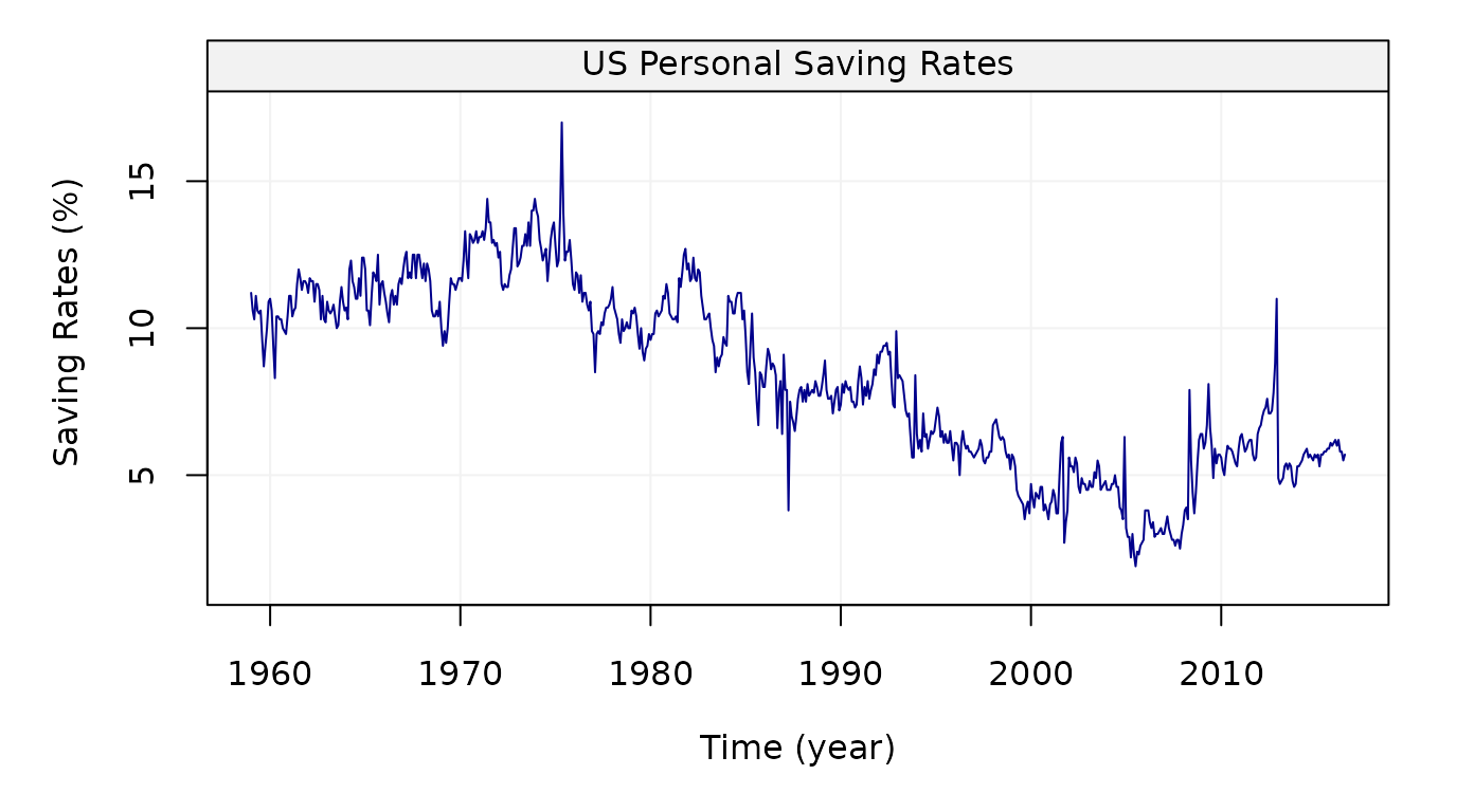

Figure 3: Monthly (seasonally adjusted) Personal Saving Rates data from January 1959 to May 2015 provided by the Federal Reserve Bank of St. Louis.

# Compute ACF and plot result
savingrt_acf = auto_corr(savingrt)
plot(savingrt_acf)

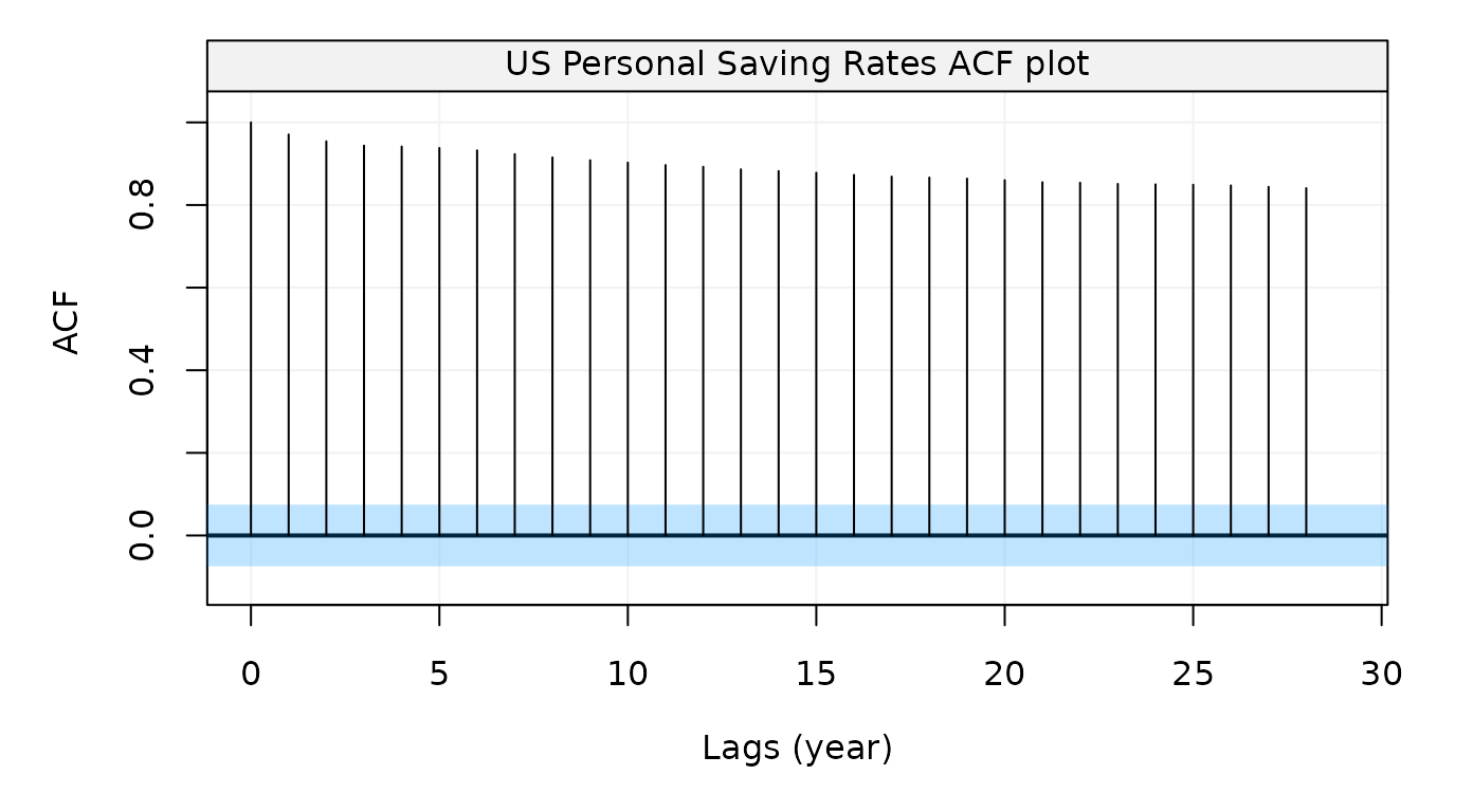
Figure 4: Empirical autocorrelation function of Personal Saving Rates data

This graph indicates that this time series is likely to present some non-stationary features. This is actually not a surprising observation as such data are often assumed to be close to a random walk model plus some (autocorrelated) noise. For this reason, let us use the GMWM to estimate a latent model given by the sum of two AR(1) models (equivalent to an ARMA(2,1) model) and a random walk.

# Estimate the latent model ARMA(2,1) + RW()
model_savings = estimate(ARMA(2,1) + RW(), savingrt, method = "gmwm")

Lynx Dataset

We can look at another dataset, lynx, annual numbers of lynx trappings in Canada for 1821-1934 in the code below:

# Load lynx dataset 
data(lynx)

# Simulate based on data
lynx = gts(as.vector(lynx), start = 1821, end = 1934, freq = 1, 
           unit_ts = bquote(paste(10^8," ",m^3)), name_ts = "Numbers", 
           unit_time = "year", data_name = "Annual Numbers of Lynx Trappings")

# Plot lynx simulation
plot(lynx)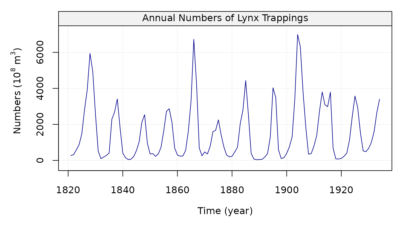

Figure 9: Plot of Annual numbers of lynx trappings for 1821-1934 in Canada

After creating the time series object, now we can compute its autocorrelation function and partial autocorrelation function by using auto_corr() as follows:

# Compute ACF and plot result
lynx_acf = auto_corr(lynx)
plot(lynx_acf)

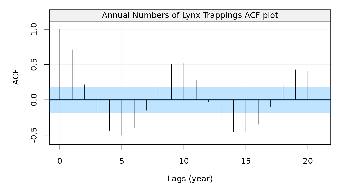
Figure 10: Empirical autocorrelation function of Annual numbers of lynx trappings in Canada for 1821-1934

# Compute PACF and plot result
lynx_pacf = auto_corr(lynx, pacf = TRUE)
plot(lynx_pacf)

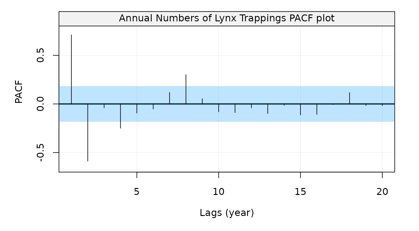
Figure 11: Empirical partial autocorrelation function of Annual numbers of lynx trappings in Canada for 1821-1934

The plot suggests some form of seasonality so one could estimate a SARMA(2,2,1) model and check its residuals as follows:

test = estimate(SARMA(2,2,1), lynx)
check(test)

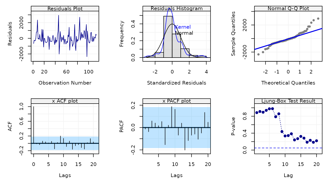
Figure 12: Empirical partial autocorrelation function of Annual numbers of lynx trappings in Canada for 1821-1934

The residuals don’t appear to follow a Gaussian distribution (first row of the plot) but there doesn’t appear to be significant dependence in them as shown in the second row of the plot showing respectively the ACF, PACF and Ljung-Box test p-values for the residuals.

Sunspot Dataset

We can look at another dataset, sunspot.year, yearly numbers of sunspots from 1700 to 1988 (rounded to one digit) in the code below:

# Load sunspot dataset 
sunspot = datasets::sunspot.year

# Simulate based on data
sunspot = gts(as.vector(sunspot.year), start = 1700, end = 1988, freq = 1, 
           unit_ts = bquote(paste(10^8," ",m^3)), name_ts = "Numbers", 
           unit_time = "year", data_name = "Yearly Numbers of Sunspots")

# Plot sunspot simulation
plot(sunspot)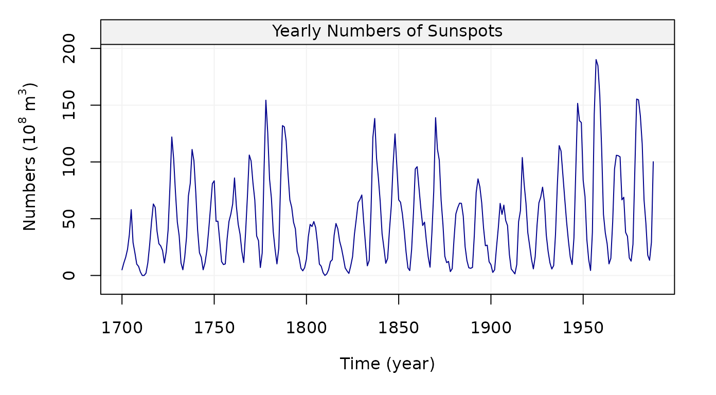

Figure 13: Plot of Yearly numbers of sunspots from 1700 to 1988

After creating the time series object, now we can compute its autocorrelation function and partial autocorrelation function by using auto_corr() as follows:

# Compute ACF and plot result
sunspot_acf = auto_corr(sunspot)
plot(sunspot_acf)

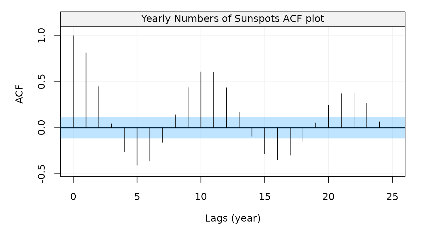
Figure 14: Empirical autocorrelation function of Yearly numbers of sunspots from 1700 to 1988

#Compute PACF and plot result
sunspot_pacf = auto_corr(sunspot, pacf = TRUE)
plot(sunspot_pacf)

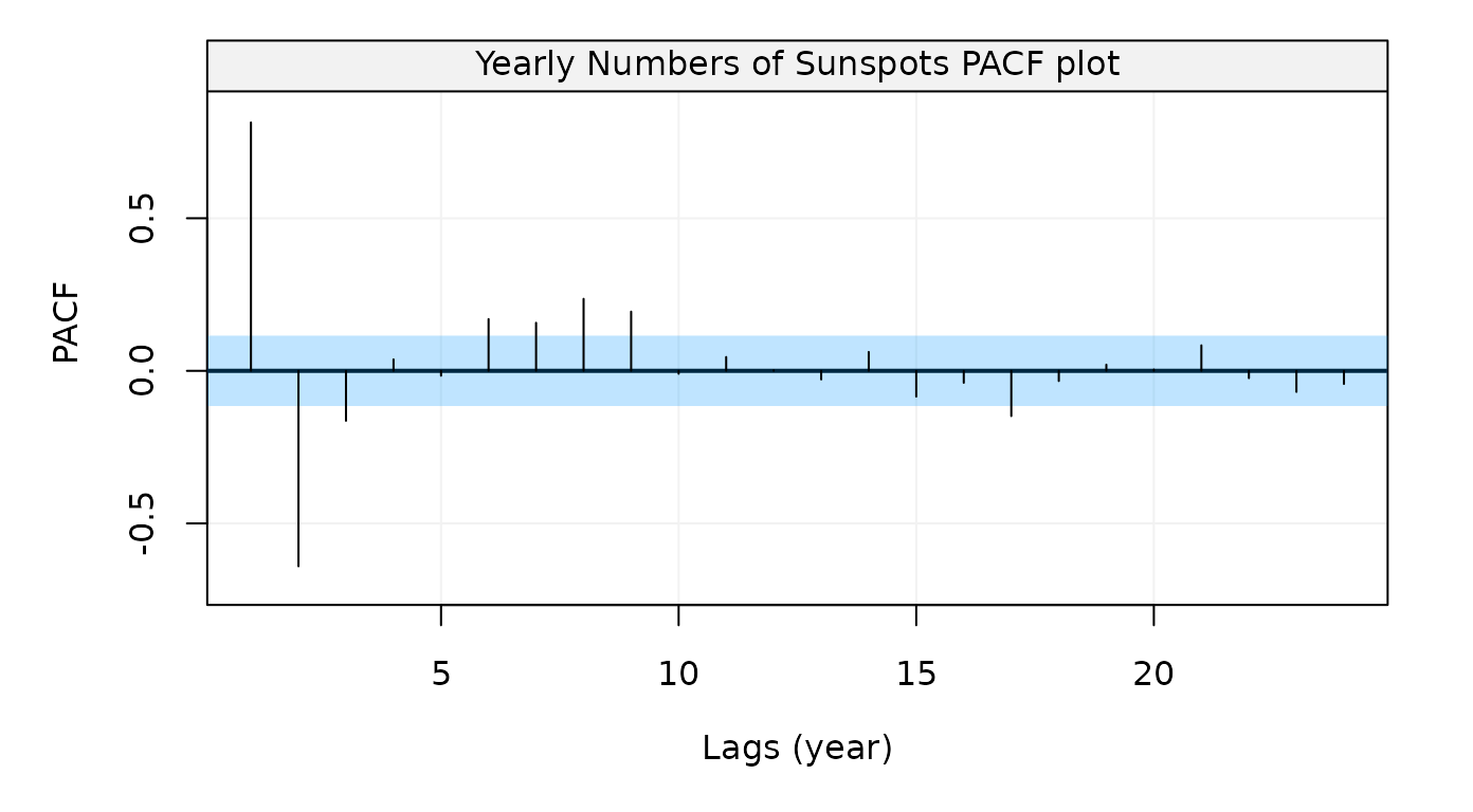
Figure 15: Empirical partial autocorrelation function of Yearly numbers of sunspots from 1700 to 1988

Let us estimate an AR(p) model and for this reason let us select the order:

select(AR(15), sunspot)

## Warning: `filter_()` was deprecated in dplyr 0.7.0.
## Please use `filter()` instead.
## See vignette('programming') for more help
## This warning is displayed once every 8 hours.
## Call `lifecycle::last_lifecycle_warnings()` to see where this warning was generated.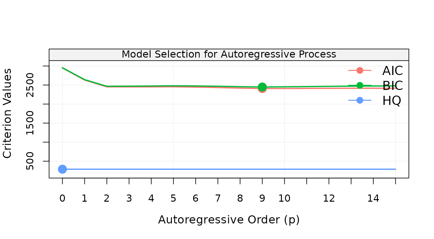

Figure 16: Results on model selection for AR(p) models for Yearly numbers of sunspots from 1700 to 1988

The results of the model selection procedure seem to indicate that the AR(9) model is the best so let us use this model to predict the future 10 observations along with their 60%, 90% and 95% confidence intervals:

model_sunspots = estimate(AR(9), sunspot)
predict(model_sunspots, n.ahead = 10, level = c(0.60, 0.90, 0.95))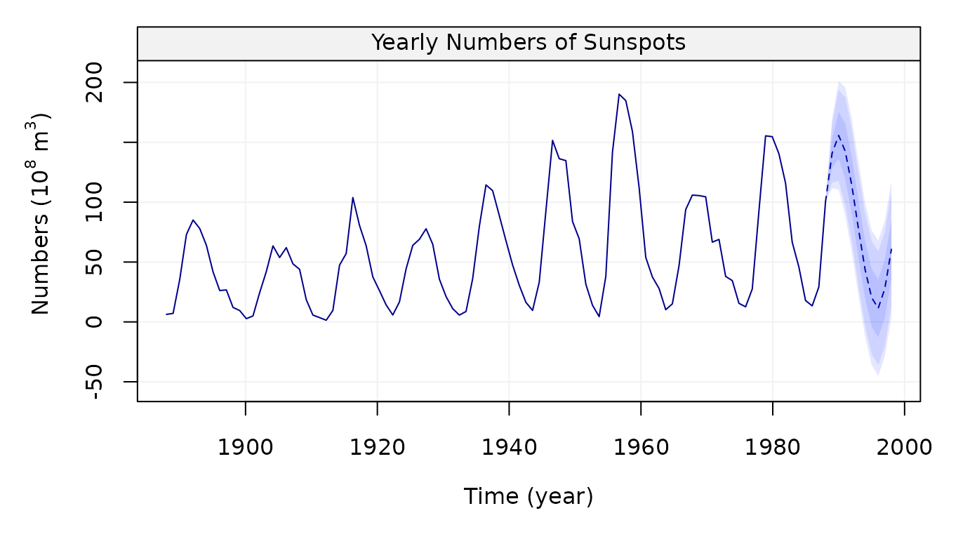

Figure 17: 10-steps-ahead forecasts (and confidence intervals) for Yearly numbers of sunspots from 1700 to 1988

Nile River Flow Dataset

Finally, we consider the last dataset, Nile, Annual Nile river flow from 1871-1970 in the code below:

# Load Nile dataset
Nile = datasets::Nile

# Simulate based on data
nile = gts(as.vector(Nile), start = 1871, end = 1970, freq = 1, 
           unit_ts = bquote(paste(10^8," ",m^3)), name_ts = "Flow", 
           unit_time = "year", data_name = "Annual Flow of the Nile River")

# Plot Nile simulation 
plot(nile)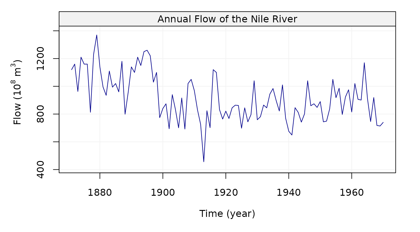

Figure 18: Plot of Annual Nile river flow from 1871-1970

To get ACF, we can use auto_corr() and make a plot:

# Compute ACF and plot result
nile_acf = auto_corr(nile)
plot(nile_acf)

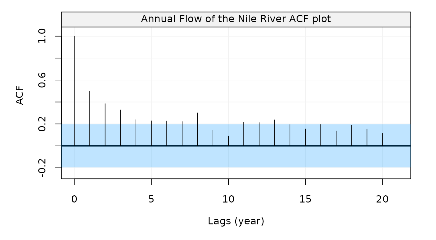
Figure 19: Empirical autocorrelation function of the Nile river flow data

Similar to the example above, we can also use corr_analysis() to get the ACF and PACF at the same time:

# Compute and plot ACF and PACF
nile_corr = corr_analysis(nile)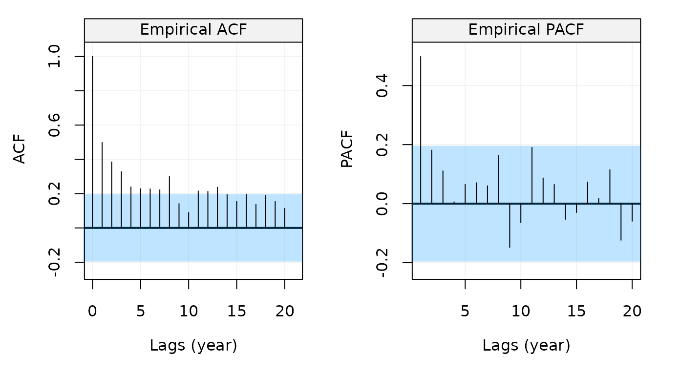

Figure 20: Empirical ACF and PACF of the Nile river flow data

# Get ACF and PACF values
nile_acf = nile_corr$ACF
nile_pacf = nile_corr$PACF

References

This package is developed mainly as a support to the online book “Applied Time Series Analysis with R”.

Cobb, George W. 1978. “The Problem of the Nile: Conditional Solution to a Changepoint Problem.” Biometrika, 243–51.

Hipel, Keith W, and A Ian McLeod. 1994. Time Series Modelling of Water Resources and Environmental Systems. Vol. 45. Elsevier.