Estimate geodetic time series with dependent errors and missing observations

Model and estimator

The gmwmx2 R package allows to estimate linear model with dependent errors described by composite stochastic model in presence of missing data.

More precisely, we assume the following model: $$\begin{equation} \boldsymbol{Y} = \boldsymbol{X} \boldsymbol{\beta} + \boldsymbol{\varepsilon}, \quad \boldsymbol{\varepsilon} \sim \mathcal{F}\left\{\boldsymbol{\Sigma}\left(\boldsymbol{\gamma}\right)\right\}, \end{equation}$$

where $\boldsymbol{X} \in \mathbb{R}^{n \times p}$ is a design matrix of observed predictors, $\boldsymbol{\beta} \in \mathbb{R}^p$ is the regression parameter vector and $\boldsymbol{\varepsilon} = \{\varepsilon_{i}\}_{i=1,\ldots,n}$ is a zero-mean process following an unspecified joint distribution $\mathcal{F}$ with positive-definite covariance function $\boldsymbol{\Sigma}(\boldsymbol{\gamma}) \in \mathbb{R}^{n\times n}$ characterizing the second-order dependence structure of the process and parameterized by the vector $\boldsymbol{\gamma} \in \boldsymbol{\Gamma} \subset \mathbb{R}^q$.

We then define the a random variable $\boldsymbol{Z} =\{Z_{i}\}_{i=1,\ldots,n}$ which describes the missing observation mechanism. More specifically, the vector $\boldsymbol{Z} \in \{0, 1\}^n$ is a binary-valued stationary process independent of $\boldsymbol{Y}$ with expectation $\mu(\boldsymbol{\vartheta}) = \mathbb{E}[Z_i] \in [0, \, 1)$, $\forall \, i$, and covariance matrix $\boldsymbol{\Lambda}(\boldsymbol{\vartheta}) = \mathbb{V}[\boldsymbol{Z}] \in \mathbb{R}^{n\times n}$ whose structure is assumed known up to the parameter vector $\boldsymbol{\vartheta} \in \boldsymbol{\Upsilon} \subset \mathbb{R}^k$

We then assume that we only observe the stochastic process $\tilde{\boldsymbol{Y}} = \boldsymbol{Z} \odot \boldsymbol{Y}$, where $\odot$ denotes the Hadamard product. Hence, $\tilde{\boldsymbol{Y}} \in \mathbb{R}^n = \boldsymbol{Y} \odot \boldsymbol{Z}$ represents the observed process vector with null elements in the positions where observations are missing.

Using $\otimes$ to denote the Kronecker product, we then define $\tilde{\boldsymbol{X}} = \boldsymbol{Z} \otimes \boldsymbol{1}^T \odot \boldsymbol{X} \in \mathbb{R}^{n \times p}$ as the design matrix $\boldsymbol{X}$ with zero-valued vectors for the rows where observations are missing in $\boldsymbol{Y}$ (where $\boldsymbol{1}$ represents a vector of ones of dimension $p$).

We estimate the parameters $\boldsymbol{\beta}$ with the least square estimator:

$$\begin{equation} \hat{\boldsymbol{\beta}} = \left(\tilde{\boldsymbol{X}}^T \tilde{\boldsymbol{X}}\right)^{-1} \tilde{\boldsymbol{X}}^T \tilde{\boldsymbol{Y}}. \end{equation}$$

We compute the estimated residuals as $\hat{\boldsymbol{\varepsilon}} = {\tilde{\boldsymbol{Y}}} - \tilde{{\boldsymbol{X}}} \hat{\boldsymbol{\beta}}$.

We then estimate with the Maximum Likelihood Estimator the parameters $\boldsymbol{\vartheta}$ of the missingness process $\boldsymbol{Z}$ assuming that $\boldsymbol{Z}$ is generated from a Markov model with the following transition probabilities:

$$\begin{equation} \label{eq:markov_model_def} \begin{aligned} & P\left( Z_2=1 \mid Z_1=1\right)=1 - p_1 \\ & P\left(Z_2=1 \mid Z_1=0\right) = p_2 \\ & P\left(Z_2=0 \mid Z_1=1\right)=p_1 \\ & P\left(Z_2=0 \mid Z_1=0\right)=1-p_2. \end{aligned} \end{equation}$$

We then estimate the parameters $\boldsymbol{\gamma}$ using a Generalized method of Wavelet Moments approach (Guerrier et al. 2013).

More precisely, we rely on the result of Xu et al. (2017) that provide a computationally efficient form of the theoretical Allan variance (equivalent to the Haar wavelet variance up to a constant) for zero-mean stochastic processes such as $\boldsymbol{\varepsilon}$ to avoid computing these large matrices multiplication in the objective function. Indeed in Xu et al. (2017) they generalize the results in Zhang (2008) to zero-mean non-stationary processes by using averages of the diagonals and super-diagonals of the covariance matrix of $\boldsymbol{\varepsilon}$. What this implies is that the GMWM, which uses this form, does not require the storage of the $n \times n$ covariance matrix of $\boldsymbol{\varepsilon}$, but only of a vector of dimension $n$ which is then plugged into an explicit formula consisting in a linear combination of the elements of this vector (these elements being averages of the diagonal and super-diagonals of the covariance matrix).

Estimating tectonic velocities and crustal uplift

While the GMWMX as described above and in more details in Voirol et al. (2024), is a general method for estimating large linear model with complex dependence structure in presence of missing data, the gmwmx2 R package is currently developed specifically to estimate tectonic velocities from position times series in graticule distance coordinates system (GD) provided by the Nevada geodetic Laboratory (Blewitt 2024; Blewitt, Hammond, and Kreemer 2018).

Trajectory model

To estimate the trajectory model (see e.g., Bevis and Brown (2014) for more details), we construct the design matrix $\boldsymbol{X}$ such that $i$-th component of the vector $\mathbf{X} {{\boldsymbol{\beta}}}$ can be described as follows with $t_i$ representing the $i^{th}$ ordered time point (epoch) indicated in Modified Julian Date and $t_0$ representing the reference epoch located exactly in the middle of start and end point of the time series:

$$\begin{split} \mathbb{E}[\mathbf{Y}_i] &= \mathbf{X}_i^T {{\boldsymbol{\beta}}} \\ &= a + b \left(t_{i} - t_0\right) + \sum_{h=1}^{m}\left[c_{h} \sin \left(2 \pi f_{h} t_{i}\right) + d_h \cos \left(2 \pi f_h t_i\right)\right] + \\& \sum_{j=1}^{r}e_j H\left(t_i - t_j\right) + \sum_{k = 1 }^{s} l_k \left[1- \exp\left(\frac{-(t_i-t_k)}{\tau_k}\right)\right]H\left(t_{i}-\tau_k\right) \end{split}$$

where $a$ is the initial position at the reference epoch $t_0$, $b$ is the velocity parameter, $c_h$ and $d_h$ are the periodic motion parameters ($h = 1$ and $h = 2$ represent the annual and semi-annual seasonal terms, respectively with $f_1 = \frac{1}{365.25}$ and $f_2 = \frac{2}{365.25}$). The offset terms models earthquakes, equipment changes or human intervention in which $e_j$ is the magnitude of the step at epochs $t_j$, $r$ is the total number of offsets, $H$ is the Heaviside step function defined as $H(x):= \begin{cases}1, & x \geq 0 \\ 0, & x<0\end{cases}$ and the last term allow to model post-seismic deformation (see e.g., Sobrero et al. (2020)) where $s$ is the number of post seismic relaxation time specified, $t_k$ is the time when the relaxation $k$ starts in Modified Julian Date (MJD), $\tau_k$ is the relaxation period in days for the post-seismic relaxation $k$ and $l_k$ is the amplitude of the transient. Note that by default the estimates of the functional parameters are provided in unit/day.

When loading data from a specific station using the function gmwmx2::download_station_ngl(), we extract from the Nevada Geodetic Laboratory the position time series in GD coordinates, the time steps associated with a equipment or software change and the time steps associated with an earthquake near the station. All these objects are stored in a object of class gnss_ts_ngl.

When applying the function gmwmx2::gmwmx2() to an object of class gnss_ts_ngl, we construct the design matrix $\boldsymbol{X}$ by considering an offset term for all equipment or software changes steps and all earthquakes indicated by the NGL. We also specify a post-seismic relaxation term for all earthquakes indicated by the NGL. If no relaxation time is specified in the argument vec_earthquakes_relaxation_time, we consider a default relaxation time of $365.25$ days.

Stochastic model

It is generally recognized that noise in GNSS time series is best described by a combination of colored noise plus white noise (He et al. 2017; Langbein 2008; Williams et al. 2004; Bos et al. 2013) where the white noise generally model noise at high frequencies and the colored noise model the lower frequencies of the spectrum.

Example of estimation

Let us showcase how to estimate the tectonic velocity in for one specific component (North, East or Vertical) of one station.

Let us first load the gmwmx2 package.

library(gmwmx2)

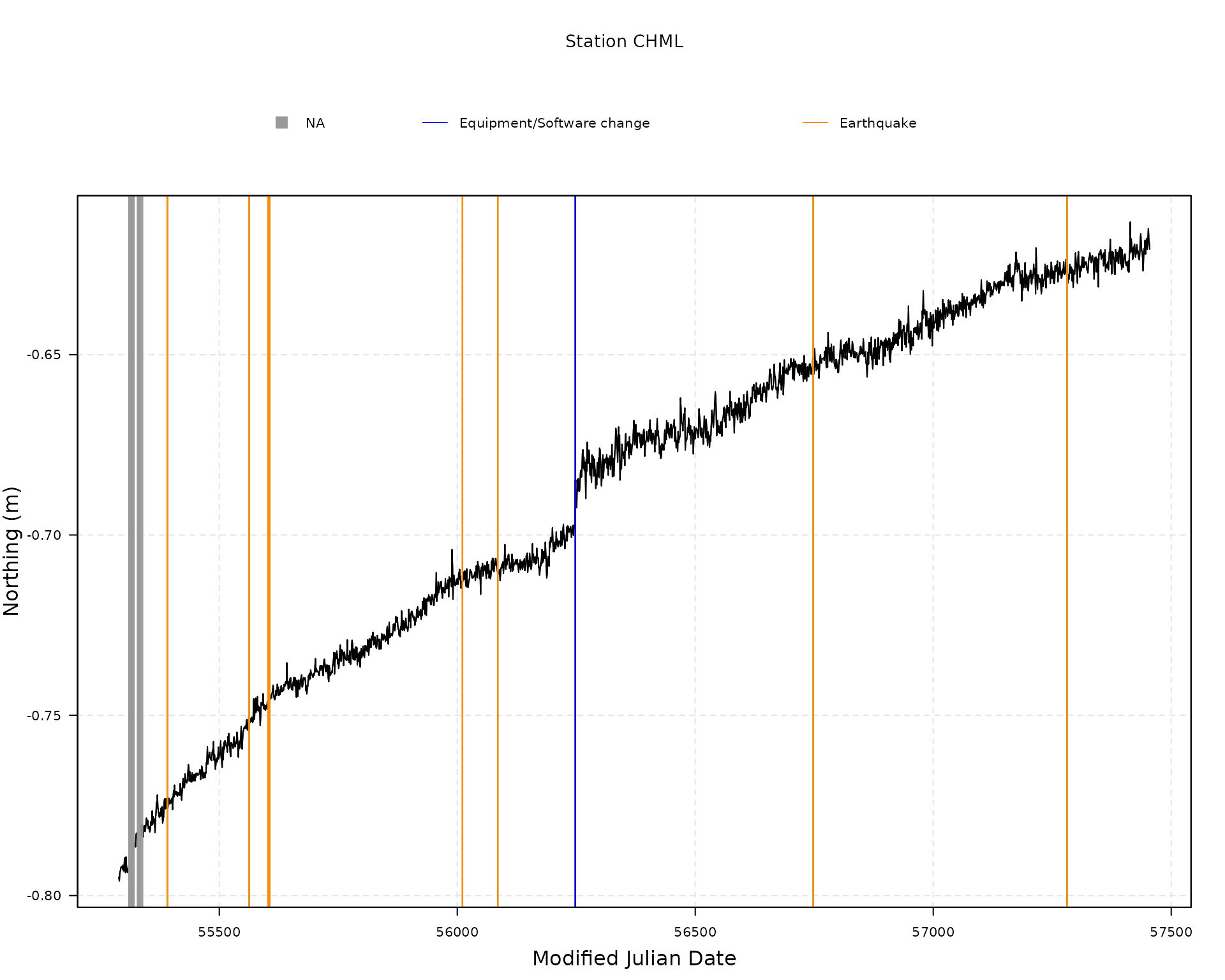
Download a station from Nevada Geodetic Laboratory

station_data <- download_station_ngl("CHML")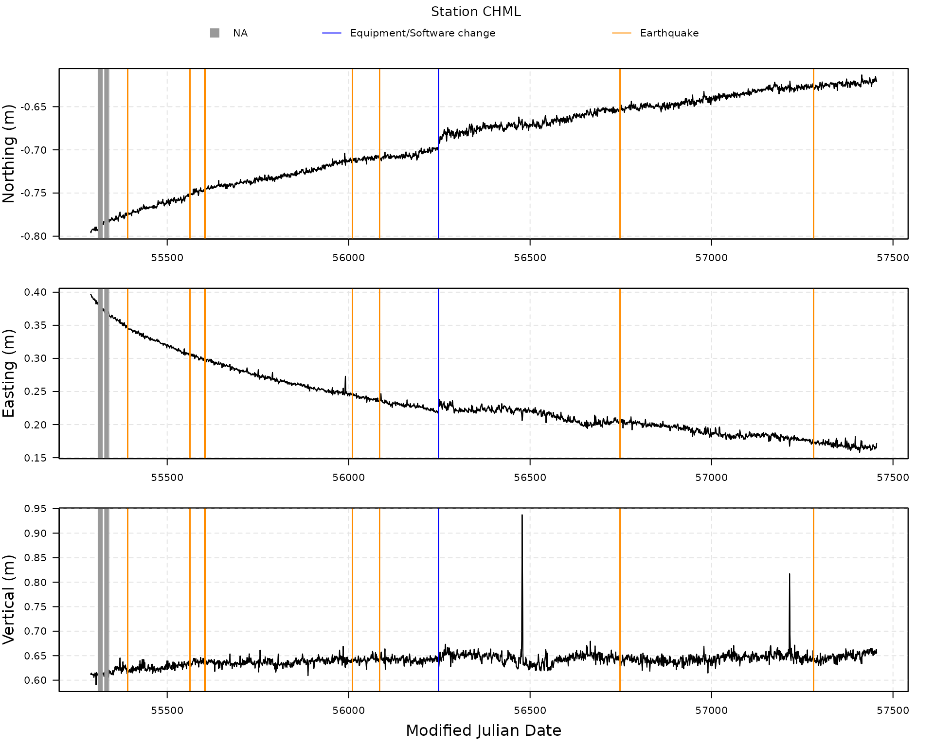

Plot Station

plot(station_data)

Plot Northing component

plot(station_data, component = "N")

Estimate model on station data

fit1 <- gmwmx2_new(station_data, n_seasonal = 2, component = "N", model = wn()+ pl())
fit1

## GMWMX fit GNSS Times Series (Nevada Geodetic Laboratory)
##                         Estimate Std.Error   CI.Lower   CI.Upper
## Intercept             -7.091e-01 7.923e-03 -7.246e-01 -6.936e-01
## Trend                  7.383e-05 7.537e-06  5.906e-05  8.860e-05
## Sin (Annual)          -6.634e-04 3.101e-04 -1.271e-03 -5.567e-05
## Cos (Annual)           7.706e-04 3.285e-04  1.268e-04  1.414e-03
## Sin (Semi-Annual)      7.358e-04 2.186e-04  3.073e-04  1.164e-03
## Cos (Semi-Annual)     -3.093e-04 2.254e-04 -7.511e-04  1.324e-04
## Jump: MJD 56248        1.698e-02 1.428e-03  1.418e-02  1.978e-02
## Jump: MJD 55391        7.543e-03 1.403e-03  4.794e-03  1.029e-02
## Jump: MJD 55563        1.638e-03 1.618e-03 -1.533e-03  4.810e-03
## Jump: MJD 55603        2.768e-03 2.214e-03 -1.570e-03  7.107e-03
## Jump: MJD 55606        7.748e-04 3.261e-03 -5.616e-03  7.166e-03
## Jump: MJD 56011       -1.185e-03 1.521e-03 -4.166e-03  1.796e-03
## Jump: MJD 56085        1.270e-03 1.561e-03 -1.789e-03  4.330e-03
## Jump: MJD 56748       -6.812e-04 1.257e-03 -3.144e-03  1.782e-03
## Jump: MJD 57281       -3.590e-04 1.404e-03 -3.110e-03  2.393e-03
## Earthquake: MJD 55391  1.819e-02 6.744e-03  4.976e-03  3.141e-02
## Earthquake: MJD 55563  9.271e-04 2.384e-02 -4.579e-02  4.765e-02
## Earthquake: MJD 55603 -3.728e-01 4.934e-01 -1.340e+00  5.942e-01
## Earthquake: MJD 55606  3.633e-01 4.879e-01 -5.929e-01  1.319e+00
## Earthquake: MJD 56011  4.511e-03 1.220e-02 -1.939e-02  2.841e-02
## Earthquake: MJD 56085 -1.898e-02 1.142e-02 -4.136e-02  3.411e-03
## Earthquake: MJD 56748 -9.572e-03 4.886e-03 -1.915e-02  4.758e-06
## Earthquake: MJD 57281 -2.302e-02 5.868e-03 -3.452e-02 -1.152e-02
## 
## Missingness model
##   Proportion missing : 0.0088 
##   p1                 : 0.0028 
##   p2                 : 0.3158 
##   p*                 : 0.9912 
## 
## Stochastic model
##   Sum of 2 processes
##   [1] White Noise
##        Estimated parameters : sigma2 = 2.987e-07 
##   [2] Stationary PowerLaw
##        Estimated parameters : kappa = -0.7261, sigma2 = 3.75e-06 
## 
## Runtime (seconds)
##   Total              : 0.8990

Plot estimated model

plot(fit1)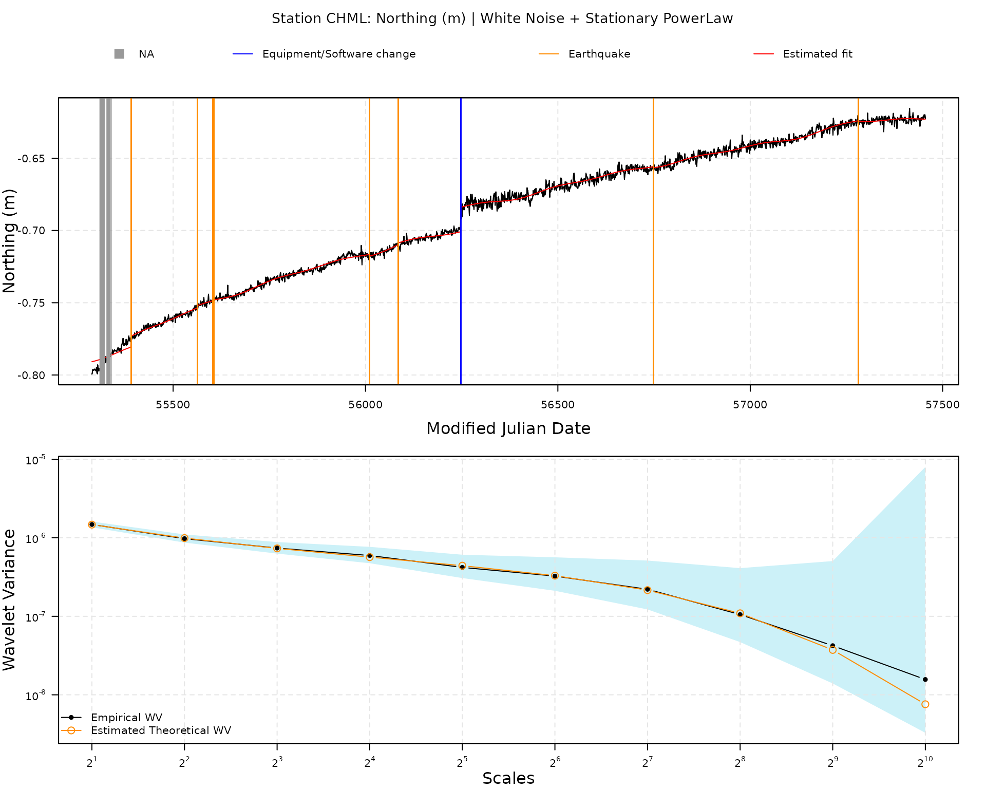

fit2 <- gmwmx2_new(station_data, n_seasonal = 2, component = "N", model = wn()+ flicker())
fit2

## GMWMX fit GNSS Times Series (Nevada Geodetic Laboratory)
##                         Estimate Std.Error   CI.Lower   CI.Upper
## Intercept             -7.091e-01 1.067e-02 -7.300e-01 -6.882e-01
## Trend                  7.383e-05 1.016e-05  5.391e-05  9.375e-05
## Sin (Annual)          -6.634e-04 4.072e-04 -1.462e-03  1.348e-04
## Cos (Annual)           7.706e-04 4.279e-04 -6.808e-05  1.609e-03
## Sin (Semi-Annual)      7.358e-04 2.609e-04  2.245e-04  1.247e-03
## Cos (Semi-Annual)     -3.093e-04 2.706e-04 -8.397e-04  2.211e-04
## Jump: MJD 56248        1.698e-02 1.800e-03  1.345e-02  2.050e-02
## Jump: MJD 55391        7.543e-03 1.716e-03  4.180e-03  1.091e-02
## Jump: MJD 55563        1.638e-03 1.781e-03 -1.854e-03  5.130e-03
## Jump: MJD 55603        2.768e-03 2.192e-03 -1.529e-03  7.065e-03
## Jump: MJD 55606        7.748e-04 3.328e-03 -5.747e-03  7.297e-03
## Jump: MJD 56011       -1.185e-03 1.806e-03 -4.726e-03  2.355e-03
## Jump: MJD 56085        1.270e-03 1.875e-03 -2.404e-03  4.945e-03
## Jump: MJD 56748       -6.812e-04 1.763e-03 -4.136e-03  2.774e-03
## Jump: MJD 57281       -3.590e-04 1.763e-03 -3.814e-03  3.096e-03
## Earthquake: MJD 55391  1.819e-02 8.731e-03  1.082e-03  3.531e-02
## Earthquake: MJD 55563  9.271e-04 2.591e-02 -4.986e-02  5.171e-02
## Earthquake: MJD 55603 -3.728e-01 4.887e-01 -1.331e+00  5.850e-01
## Earthquake: MJD 55606  3.633e-01 4.833e-01 -5.839e-01  1.310e+00
## Earthquake: MJD 56011  4.511e-03 1.414e-02 -2.321e-02  3.223e-02
## Earthquake: MJD 56085 -1.898e-02 1.364e-02 -4.570e-02  7.752e-03
## Earthquake: MJD 56748 -9.572e-03 6.809e-03 -2.292e-02  3.774e-03
## Earthquake: MJD 57281 -2.302e-02 7.612e-03 -3.794e-02 -8.102e-03
## 
## Missingness model
##   Proportion missing : 0.0088 
##   p1                 : 0.0028 
##   p2                 : 0.3158 
##   p*                 : 0.9912 
## 
## Stochastic model
##   Sum of 2 processes
##   [1] White Noise
##        Estimated parameters : sigma2 = 1.736e-06 
##   [2] Flicker
##        Estimated parameters : sigma2 = 2.062e-06 
## 
## Runtime (seconds)
##   Total              : 0.5066

plot(fit2)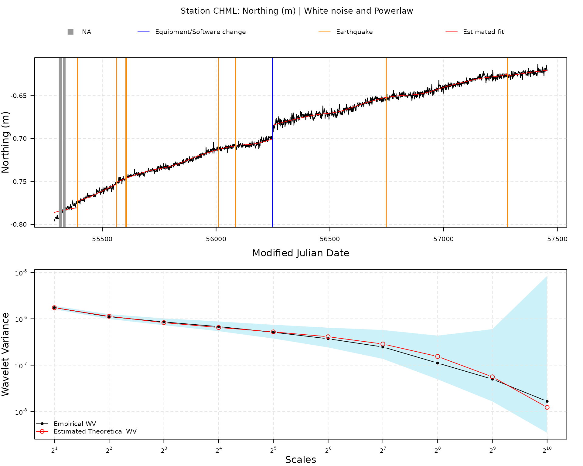

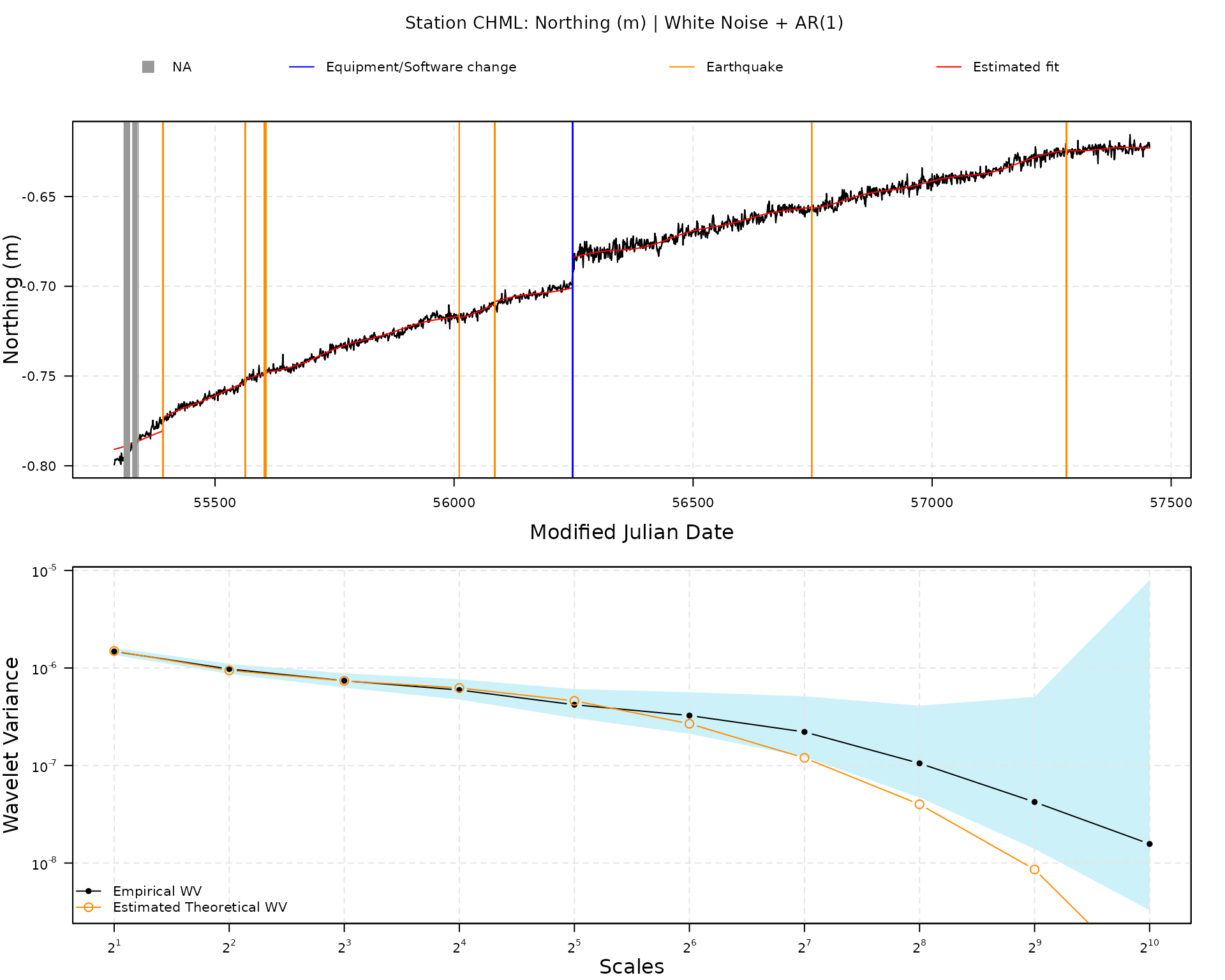
fit3 = gmwmx2_new(station_data, n_seasonal = 2, component = "N", model = wn() + ar1())
fit3

## GMWMX fit GNSS Times Series (Nevada Geodetic Laboratory)
##                         Estimate Std.Error   CI.Lower   CI.Upper
## Intercept             -7.091e-01 4.350e-03 -7.176e-01 -7.006e-01
## Trend                  7.383e-05 4.156e-06  6.568e-05  8.198e-05
## Sin (Annual)          -6.634e-04 1.746e-04 -1.006e-03 -3.211e-04
## Cos (Annual)           7.706e-04 1.892e-04  3.998e-04  1.141e-03
## Sin (Semi-Annual)      7.358e-04 1.575e-04  4.272e-04  1.044e-03
## Cos (Semi-Annual)     -3.093e-04 1.604e-04 -6.236e-04  4.957e-06
## Jump: MJD 56248        1.698e-02 9.445e-04  1.513e-02  1.883e-02
## Jump: MJD 55391        7.543e-03 9.571e-04  5.667e-03  9.419e-03
## Jump: MJD 55563        1.638e-03 1.461e-03 -1.226e-03  4.502e-03
## Jump: MJD 55603        2.768e-03 2.220e-03 -1.583e-03  7.119e-03
## Jump: MJD 55606        7.748e-04 3.132e-03 -5.364e-03  6.913e-03
## Jump: MJD 56011       -1.185e-03 1.172e-03 -3.482e-03  1.112e-03
## Jump: MJD 56085        1.270e-03 1.193e-03 -1.068e-03  3.609e-03
## Jump: MJD 56748       -6.812e-04 6.133e-04 -1.883e-03  5.209e-04
## Jump: MJD 57281       -3.590e-04 9.322e-04 -2.186e-03  1.468e-03
## Earthquake: MJD 55391  1.819e-02 4.112e-03  1.014e-02  2.625e-02
## Earthquake: MJD 55563  9.271e-04 2.214e-02 -4.246e-02  4.432e-02
## Earthquake: MJD 55603 -3.728e-01 4.842e-01 -1.322e+00  5.762e-01
## Earthquake: MJD 55606  3.633e-01 4.786e-01 -5.748e-01  1.301e+00
## Earthquake: MJD 56011  4.511e-03 9.924e-03 -1.494e-02  2.396e-02
## Earthquake: MJD 56085 -1.898e-02 8.742e-03 -3.611e-02 -1.842e-03
## Earthquake: MJD 56748 -9.572e-03 2.435e-03 -1.435e-02 -4.799e-03
## Earthquake: MJD 57281 -2.302e-02 3.566e-03 -3.001e-02 -1.603e-02
## 
## Missingness model
##   Proportion missing : 0.0088 
##   p1                 : 0.0028 
##   p2                 : 0.3158 
##   p*                 : 0.9912 
## 
## Stochastic model
##   Sum of 2 processes
##   [1] White Noise
##        Estimated parameters : sigma2 = 2.469e-06 
##   [2] AR(1)
##        Estimated parameters : phi = 0.782, sigma2 = 9.644e-07 
## 
## Runtime (seconds)
##   Total              : 0.1925

plot(fit3)

References

Bevis, Michael, and A. Brown. 2014. “Trajectory models and reference frames for crustal motion geodesy.” Journal of Geodesy 88 (283): 283--311. https://doi.org/10.1007/s00190-013-0685-5.

Blewitt, Geoffrey. 2024. “An Improved Equation of Latitude and a Global System of Graticule Distance Coordinates.” Journal of Geodesy 98 (1): 6.

Blewitt, Geoffrey, William Hammond, and Corn Kreemer. 2018. “Harnessing the GPS Data Explosion for Interdisciplinary Science.” Eos 99 (2): e2020943118.

Bos, MS, RMS Fernandes, SDP Williams, and L Bastos. 2013. “Fast Error Analysis of Continuous GNSS Observations with Missing Data.” Journal of Geodesy 87 (4): 351–60.

Guerrier, Stéphane, Jan Skaloud, Yannick Stebler, and Maria-Pia Victoria-Feser. 2013. “Wavelet-Variance-based Estimation for Composite Stochastic Processes.” Journal of the American Statistical Association 108 (503): 1021–30.

He, Xiaoxing, Jean-Philippe Montillet, Rui Fernandes, Machiel Bos, Kegen Yu, Xianghong Hua, and Weiping Jiang. 2017. “Review of Current GPS Methodologies for Producing Accurate Time Series and their Error Sources.” Journal of Geodynamics 106: 12–29.

Langbein, John. 2008. “Noise in GPS Displacement Measurements from Southern California and Southern Nevada.” Journal of Geophysical Research: Solid Earth 113 (B5): 1–12.

Sobrero, Franco S, Michael Bevis, Demián D Gómez, and Fei Wang. 2020. “Logarithmic and Exponential Transients in GNSS Trajectory Models as Indicators of Dominant Processes in Postseismic Deformation.” Journal of Geodesy 94 (9): 84.

Voirol, Lionel, Haotian Xu, Yuming Zhang, Luca Insolia, Roberto Molinari, and Stéphane Guerrier. 2024. “Inference for Large Scale Regression Models with Dependent Errors.” arXiv Preprint arXiv:2409.05160.

Williams, Simon DP, Yehuda Bock, Peng Fang, Paul Jamason, Rosanne M Nikolaidis, Linette Prawirodirdjo, Meghan Miller, and Daniel J Johnson. 2004. “Error Analysis of Continuous GPS Position Time Series.” Journal of Geophysical Research: Solid Earth 109 (B3).

Xu, Haotian, Stéphane Guerrier, Roberto Molinari, and Yuming Zhang. 2017. “A Study of the Allan Variance for Constant-mean Nonstationary Processes.” IEEE Signal Processing Letters 24 (8): 1257–60.

Zhang, Nien Fan. 2008. “Allan Variance of Time Series Models for Measurement Data.” Metrologia 45 (5): 549.