Generate data from a model

# libraries
library(simts)
library(gmwmx)

phase =     0.45
amplitude = 2.5
sigma2_wn =       15
sigma2_powerlaw = 10
d =               0.4
bias =            0
trend =           5/365.25
cosU =            amplitude*cos(phase)
sinU =            amplitude*sin(phase)

Let us consider a period of 5 year with daily observations:

n = 5*365

Using functions implemented in simts, we generate realizations from the sum of a White noise and PowerLaw process.

Note that the functions that enable to generate stochastic models that include Power Law process, Matèrn process or Fractional Gaussian noise are (for now) only available from the development version of the package simts that can be easily installed with:

install.packages("devtools")
devtools::install_github("SMAC-Group/simts")

model_i = WN(sigma2 = sigma2_wn) + PLP(sigma2 = sigma2_powerlaw, d = d)

# define time at which there are jumps
jump_vec =  c(600, 1200)
jump_height = c(20, 30)

# define myseed
myseed=123

We generate residuals from the stochastic model

# generate residuals
eps = simts::gen_gts(model = model_i, n= n)

Using function create_A_matrix(), we encode the intercept, a deterministic vector (trend) and sinusoidal signals in a matrix $\boldsymbol{A}$ in order to compute the deterministic component of the signal in a linear fashion. Similarly, we define the vector of fixed coefficients denoted by $\boldsymbol{x}_0$ in the paper.

# add trend and sin
A = gmwmx::create_A_matrix(t_nogap = 1:length(eps), n_seasonal =  1, jumps = NULL)

# define beta
x_0 = c(bias, trend,  cosU,  sinU)
  
# create time series
deterministic_signal = A %*% x_0

We can graphically represent the functional and stochastic component of the model as follows

plot(deterministic_signal, type="l")

plot(eps)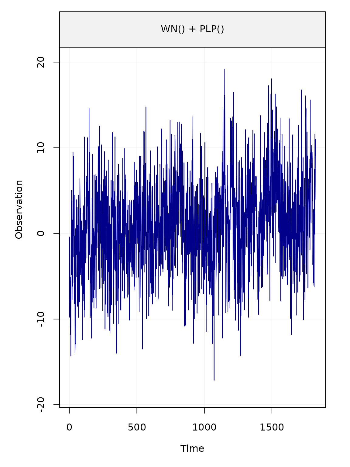

We can add location shifts (jumps) in the signal as such:

# add trend, gaps and sin
A = gmwmx::create_A_matrix(t_nogap = 1:length(eps), n_seasonal =  1, jumps = jump_vec)

# define beta
x_0 = c(bias, trend,  cosU,  sinU, jump_height)
  
# create time series
deterministic_signal = A %*% x_0

plot(deterministic_signal, type="l")

plot(eps)

We can then define and plot the generated time series

yy = deterministic_signal + eps
plot(yy)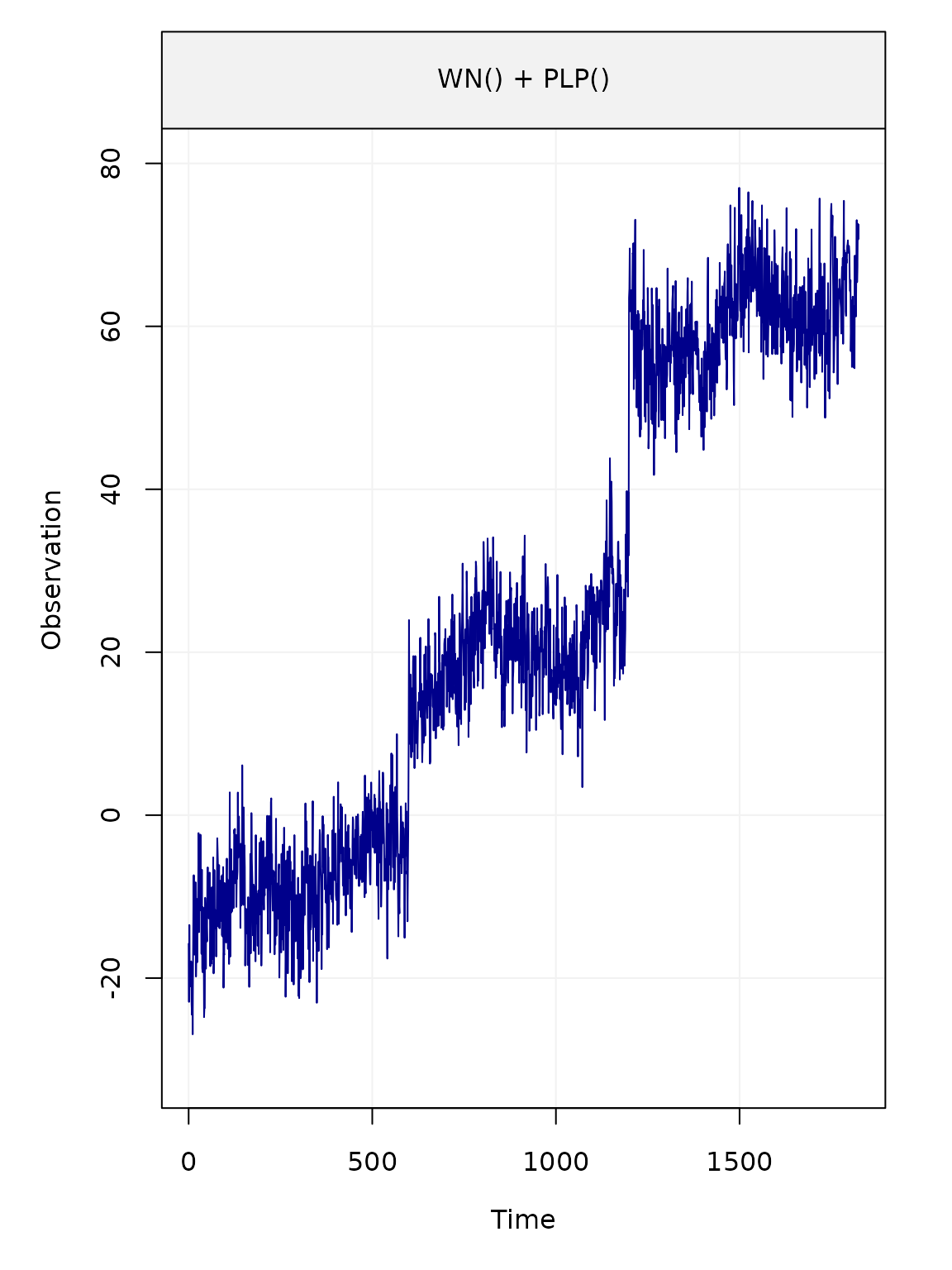

We define a gnssts object.

# save signal in temp
gnssts_obj = create.gnssts(t = 1:length(yy), y = yy, jumps = jump_vec)

class(gnssts_obj)
#> [1] "gnssts"

We can save a gnssts object as a .mom file with the function write.gnssts()

write.gnssts(gnssts_obj, filename = "simulated_data.mom")

The saved .mom file will have the following structure:

# sampling period 1.000000
# offset 100.000000
# offset 200.000000
1 9.89397119231205
2 8.52434609242207
3 9.32563441388655
4 13.4598690226589
5 8.21468271071893
6 -1.62924569468478
7 17.8036063408026
8 7.13794134326489
9 5.34700832531847

fit_gmwmx = gmwmx::estimate_gmwmx(x = gnssts_obj,
                                  model_string = "wn+powerlaw",
                                  n_seasonal = 1,
                                  theta_0 = c(0.1, 0.1, 0.1),
                                  k_iter = 1)

fit_gmwmx
#> GNSS time series model
#> 
#>  * Model: wn + powerlaw 
#> 
#>  * Functional parameters:
#>      bias            :  +0.778520
#>      trend           :  +0.015804
#>      A*cos(U)        :  +2.366464
#>      A*sin(U)        :  +1.958204
#>      jump            : +20.061620
#>      jump            : +30.596085
#> 
#>  * Stochastic parameters:
#>      wn_sigma2                      :    +11.80775096
#>      powerlaw_sigma2                :    +11.93347935
#>      powerlaw_d                     :     +0.34017417
#> 
#>  * Estimation time: 0.19 s
plot(fit_gmwmx)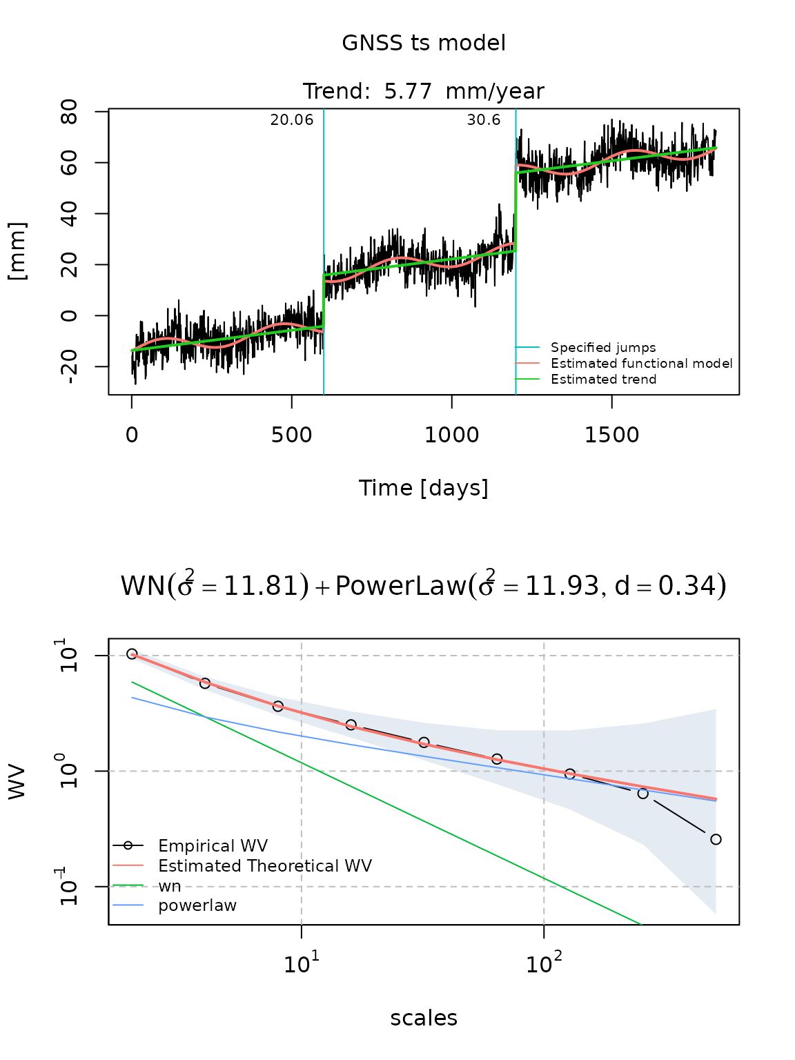

fit_gmwmx_2 = gmwmx::estimate_gmwmx(x = gnssts_obj,
                                    model_string = "wn+powerlaw",
                                    n_seasonal = 1,
                                    theta_0 = c(0.1, 0.1, 0.1),
                                    k_iter = 2)

fit_gmwmx_2
#> GNSS time series model
#> 
#>  * Model: wn + powerlaw 
#> 
#>  * Functional parameters:
#>      bias            :  +0.891683
#>      trend           :  +0.016483
#>      A*cos(U)        :  +2.438139
#>      A*sin(U)        :  +2.043069
#>      jump            : +19.550541
#>      jump            : +30.869573
#> 
#>  * Stochastic parameters:
#>      wn_sigma2                      :    +11.96947053
#>      powerlaw_sigma2                :    +11.75061286
#>      powerlaw_d                     :     +0.34298983
#> 
#>  * Estimation time: 0.49 s
plot(fit_gmwmx_2)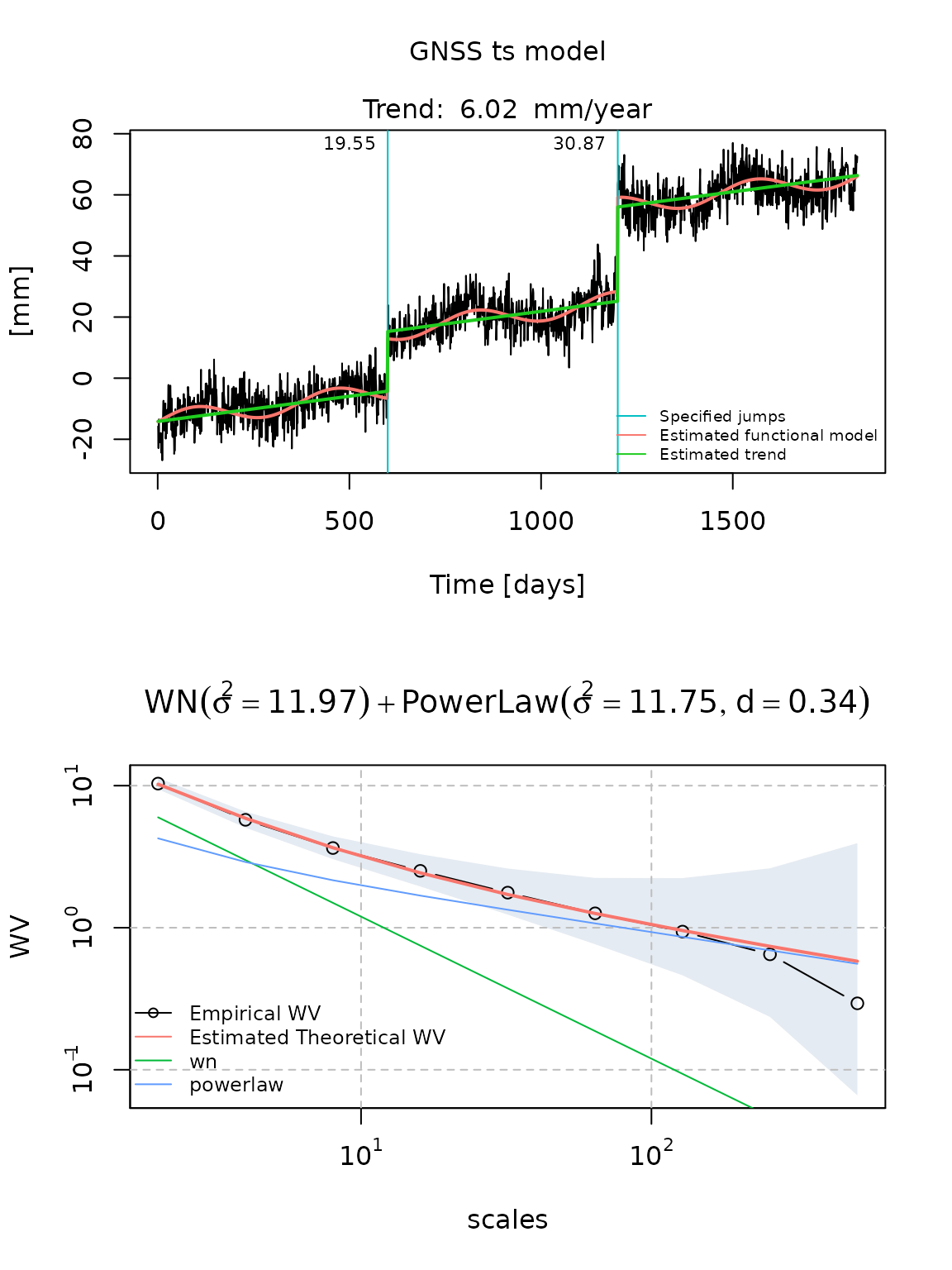

fit_mle_hector = gmwmx::estimate_hector(x = gnssts_obj,
                                    model_string = "wn+powerlaw",
                                    n_seasonal = 1
                                    )

fit_mle_hector
#> GNSS time series model
#> 
#>  * Model: wn + powerlaw 
#> 
#>  * Functional parameters:
#>      bias            :  -0.889000 +/- 1.5900000000
#>      trend           :  +0.015639 +/- 0.0019873265
#>      A*cos(U)        :  +2.542700 +/- 0.4870740000
#>      A*sin(U)        :  +0.966218 +/- 0.4826000000
#>      jump            : +18.008400 +/- 1.5199300000
#>      jump            : +30.626100 +/- 1.5310600000
#> 
#>  * Stochastic parameters:
#>      wn_sigma2                      :     +9.10561714
#>      powerlaw_sigma2                :    +17.73165228
#>      powerlaw_d                     :     +0.29703100
#> 
#>  * Estimation time: 20.17 s
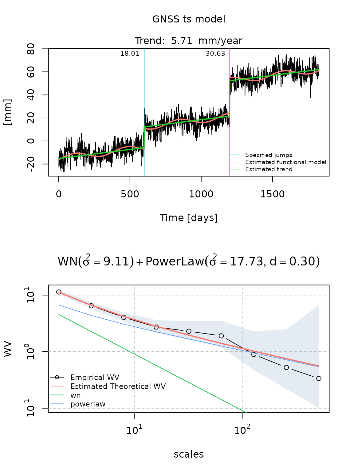
plot(fit_mle_hector)