Remove extreme values in a time series signal with Hector

# libraries
library(simts)
library(gmwmx)

phase =     0.45
amplitude = 2.5
sigma2_wn =       15
sigma2_powerlaw = 10
d =               0.4
bias =            0
trend =           5/365.25
cosU =            amplitude*cos(phase)
sinU =            amplitude*sin(phase)

# generate model
N = c(1, 7.5, 10, 15, 20)*365

# consider 2 year of data
n = N[1]
model_i = WN(sigma2 = sigma2_wn) 

# define time at which there are jumps
jump_vec =  c(100, 200)
jump_height = c(10, 20)

# define myseed
myseed=123

# set seed
set.seed(myseed)

# generate residuals
eps = simts::gen_gts(model = model_i, n= n)

# add trend, gaps and sin
A = gmwmx::create_A_matrix(1:length(eps), jump_vec, n_seasonal =  1)

# define beta
x_0 = c(bias, trend, jump_height,  cosU,  sinU)

# create time series
yy = A %*% x_0 + eps

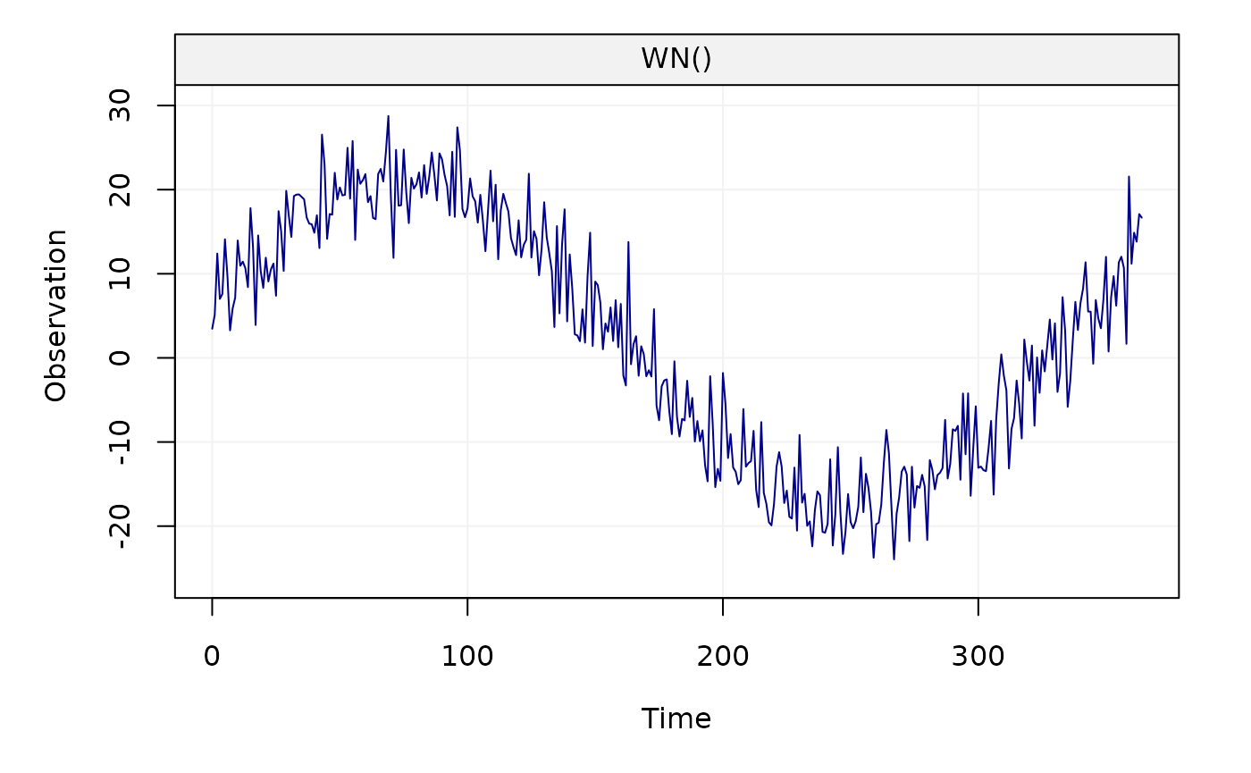
We plot the generated time series

plot(yy)

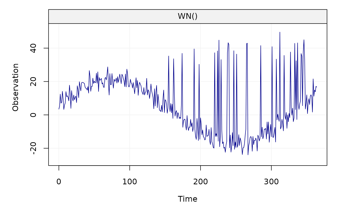
We add extreme values in the signal

n_outliers = 30
set.seed(123)
id_outliers=sample(150:350, size = n_outliers)
val_outliers = rnorm(n = n_outliers, mean = max(yy)+10, sd = 5)
yy[id_outliers] = val_outliers

We plot the corrupted time series

plot(yy)

We create a gnssts object

# save signal in temp
gnssts_obj = create.gnssts(t = 1:length(yy), y = yy, jumps = jump_vec)

We remove extreme values from the signal using removeoutliers function of Hector available by calling remove_outliers_hector()

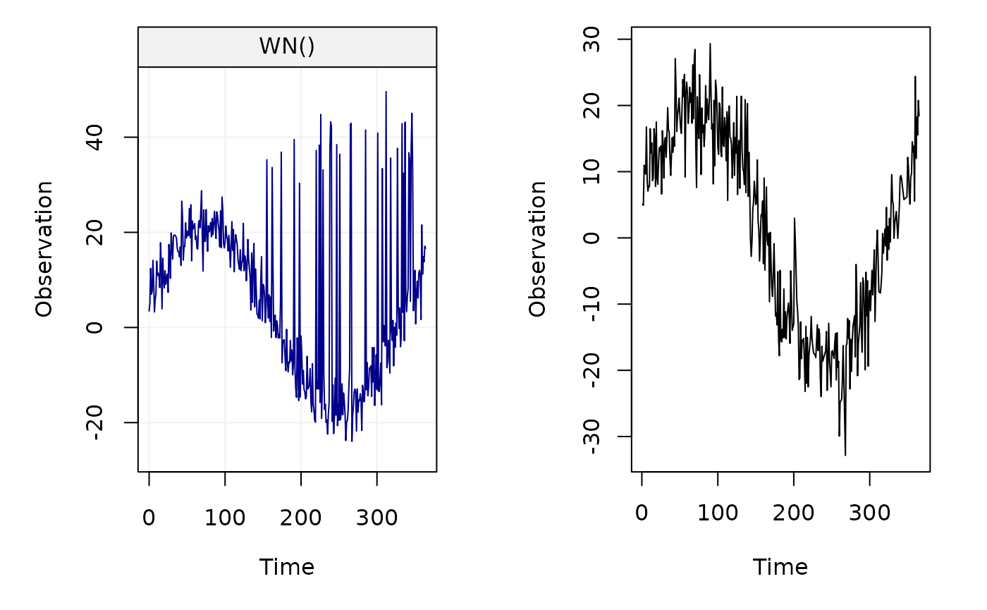
clean_yy = remove_outliers_hector(x=gnssts_obj, n_seasonal = 1)

We can compare the original and the signal with detected extreme values removed from the signal:

par(mfrow=c(1,2))
plot(yy)
plot(clean_yy$t, clean_yy$y, type = "l", xlab="Time", ylab = "Observation")