Load data, estimate and compare models

Importing a `.mom` file as a `gnssts` object

Let us first load the gmwmx package.

library(gmwmx)

Consider that you want to estimate a model on data saved in a .mom file located at a specific file_path on your computer, where file_path is the path where is located the .mom file (for example file_path = "/home/name_of_the_user/Documents/data.mom")

For example, the corresponding .mom file could have a similar looking:

# sampling period 1.000000
# offset 55285.000000
# offset 58287.770833
52759.5 -0.01165
52760.5 -0.01102
52761.5 -0.01147
...

You can import the .mom file as a with the function read.gnssts() as such:

data_dobs = read.gnssts(filename = file_path)

Objects created or imported with create.gnss() or read.gnssts() are of class gnssts.

class(data_dobs)

## [1] "gnssts"

By inspecting the structure of a gnssts object, we observe that gnssts objects specify the time vector, the observation vector, the sampling period and the times at which there are location shifts (jumps).

str(data_dobs)

## List of 4
##  $ t              : num [1:5559] 52760 52760 52762 52764 52766 ...
##  $ y              : num [1:5559] -0.0117 -0.011 -0.0115 -0.0131 -0.0106 ...
##  $ sampling_period: num 1
##  $ jumps          : num [1:2] 55285 58288
##  - attr(*, "class")= chr "gnssts"

We can represent the signal as such:

plot(data_dobs$t, data_dobs$y, type="l")

Estimate a model

Supported models

The gmwmx package allows to estimate linear model with correlated residuals that are described by a functional model and a stochastic noise model.

Functional model

More precisely, for the functional model, we consider a linear model which can be expressed as:

\[\begin{equation} \mathbf{Y} = \mathbf{A} {{\bf x}}_0 + \boldsymbol{\varepsilon}, \end{equation}\]

where \(\mathbf{Y} \in {\rm I\!R}^n\) denotes the response variable of interest (i.e., vector of GNSS observations), \(\mathbf{A} \in {\rm I\!R}^{n \times p}\) a fixed design matrix, \({{\bf x}}_0 \in \mathcal{X} \subset {\rm I\!R}^p\) a vector of unknown constants and \(\boldsymbol{\varepsilon} \in {\rm I\!R}^n\) a vector of (zero mean) residuals.

The gmwmx package allows to estimate functional models for which the \(i\)-th component of the vector \(\mathbf{A} {{\bf x}}_0\) can be described as follows:

\[\begin{equation} \mathbb{E}[\mathbf{Y}_i] = \mathbf{A}_i^T {{\bf x}}_0 = a+b\left(t_{i}-t_{0}\right)+\sum_{h=1}^{2}\left[c_{h} \sin \left(2 \pi f_{h} t_{i}\right)+d_{h} \cos \left(2 \pi f_{h} t_{i}\right)\right] + \sum_{k=1}^{n_{g}} g_{k} H\left(t_{i}-t_{k}\right), \end{equation}\]

where \(a\) is the initial position at the reference epoch \(t_0\), \(b\) is the velocity parameter, \(c_k\) and \(d_k\) are the periodic motion parameters (\(h = 1\) and \(h = 2\) represent the annual and semi-annual seasonal terms, respectively). The offset terms models earthquakes, equipment changes or human intervention in which \(g_k\) is the magnitude of the change at epochs \(t_k\), \(n_g\) is the total number of offsets, and \(H\) is the Heaviside step function. Note that the estimates of the parameters of the functional model are provided in unit/day.

Stochastic model

Regarding the stochastic model, we assume that \(\boldsymbol{\varepsilon}_i=\mathbf{Y}_i-\mathbb{E}[\mathbf{Y}_i]\) is a strictly (intrinsically) stationary process and that

\[\begin{equation} \boldsymbol{\varepsilon} \sim \mathcal{F} \left\{\mathbf{0}, \boldsymbol{\Sigma}(\boldsymbol{\gamma}_0)\right\} , \label{eq:model:noise} \end{equation}\]

where \(\mathcal{F}\) denotes some probability distribution in \({\rm I\!R}^n\) with mean \({\bf 0}\) and covariance \(\boldsymbol{\Sigma}(\boldsymbol{\gamma}_0)\).

We assume that \(\boldsymbol{\Sigma}(\boldsymbol{\gamma}_0) > 0\) and that it depends on the unknown parameter vector \(\boldsymbol{\gamma}_0 \in \boldsymbol{\Gamma} \subset {\rm I\!R}^q\). This parameter vector specifies the covariance of the observations and is often referred to as the stochastic parameters.

Hence, we let \(\boldsymbol{\theta}_0 = \left[\boldsymbol{{\bf x}}_0^{\rm T} \;\; \boldsymbol{\gamma}_0^{\rm T}\right]^{\rm T} \in \boldsymbol{\Theta} = \mathcal{X} \times \boldsymbol{\Gamma} \subset {\rm I\!R}^{p + k}\) denote the unknown parameter vector of the model described above.

The gmwmx allows to estimate parameters of a specified functional model as well as parameters of a stochastic model (i.e. \(\hat{\boldsymbol{\theta}} = \left[\boldsymbol{\hat{\boldsymbol{x}}}^{T} \;\; \hat{\boldsymbol{\gamma}}^{T}\right]\)) defined by a combinations of

White noise (wn)
Matérn process (matern)
Fractional Gaussian noise (fgn) and
Power Law process (powerlaw).

Note that only the gmwmx current version accepts only one process of each kind.

Estimate a model with the GMWMX

You can estimate a model using the GMWMX estimator with the function estimate_gmwmx().

The stochastic model considered is specified by a string provided to the argument model_string which is a combination of the strings wn, powerlaw, matern and fgn separated by the character +.

You specify the initialization values for solving the optimization problem at the GMWM estimation step that estimate the stochastic model by providing a numeric vector of the correct length (the total number of parameters of the stochastic model specified in model_string) to the argument theta_0.

You can compute confidence intervals for estimated functional parameters of an estimated model by setting the argument ci to TRUE.

Let us consider a single sinusoidal signal with the jumps specified in the gnssts object and a combination of a White noise and a Power Law process for the stochastic model.

fit_dobs_wn_plp_gmwmx = estimate_gmwmx(x = data_dobs, theta_0 = c(0.1, 0.1, 0.1), 
                                       model_string = "wn+powerlaw", 
                                       n_seasonal = 1, ci = T)

Estimated models are of class gnsstsmodel

class(fit_dobs_wn_plp_gmwmx)

## [1] "gnsstsmodel"

We can print the estimated model or extract estimated parameters (functional and stochastic) as such:

print(fit_dobs_wn_plp_gmwmx)

## GNSS time series model
## 
##  * Model: wn + powerlaw 
## 
##  * Functional parameters:
##      bias            :  +0.012013 +/- 0.0200366449
##      trend           :  +0.000008 +/- 0.0000001991
##      A*cos(U)        :  -0.000655 +/- 0.0000754528
##      A*sin(U)        :  +0.000016 +/- 0.0000762463
##      jump            :  -0.003758 +/- 0.0005738092
##      jump            :  +0.001568 +/- 0.0006045750
## 
##  * Stochastic parameters:
##      wn_sigma2                      :     +0.00000079
##      powerlaw_sigma2                :     +0.00000025
##      powerlaw_d                     :     +0.49990000
## 
##  * Estimation time: 1.66 s

fit_dobs_wn_plp_gmwmx$beta_hat

##          bias         trend      A*cos(U)      A*sin(U)          jump 
##  1.201297e-02  8.351512e-06 -6.553985e-04  1.578605e-05 -3.758074e-03 
##          jump 
##  1.567881e-03

fit_dobs_wn_plp_gmwmx$theta_hat

##       wn_sigma2 powerlaw_sigma2      powerlaw_d 
##    7.916985e-07    2.525867e-07    4.999000e-01

We can also plot graphically the estimated functional model on the time series and the Wavelet variance of residuals by calling the plot.gnsstsmodel method on a gnsstsmodel object.

plot(fit_dobs_wn_plp_gmwmx)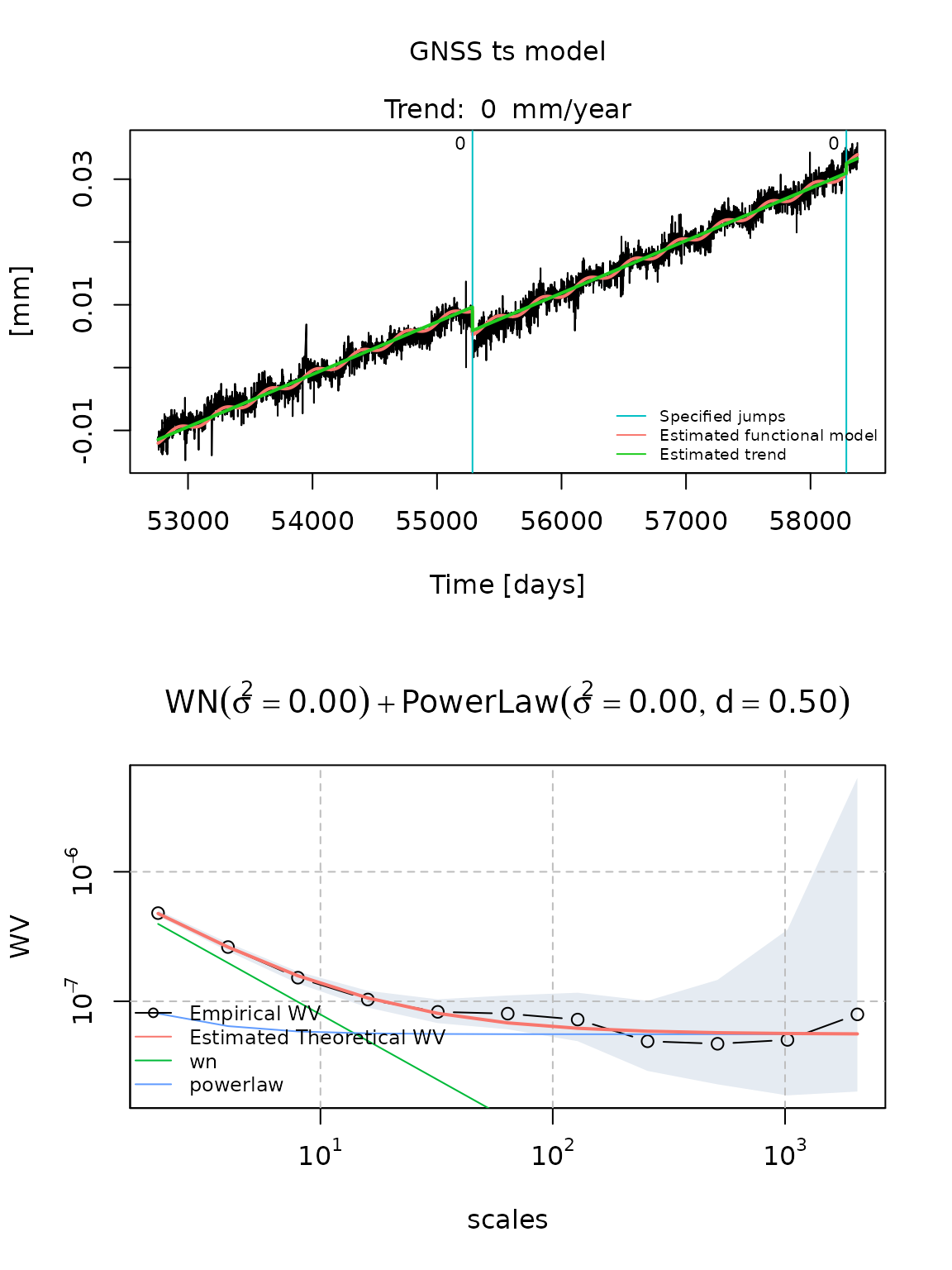

We can specify the number of iterations of the GMWMX to compute respectively the GMWMX-1 and GMWMX-2 or other iteration of the GMWMX with the argument k_iter. For example we can compute the GMWMX-2 as such:

fit_dobs_wn_plp_gmwmx_2 = estimate_gmwmx(x = data_dobs,
                                         theta_0 = c(0.1, 0.1, 0.1), 
                                         model_string = "wn+powerlaw",
                                         n_seasonal = 1, 
                                         k_iter = 2)

Estimate a model with the MLE implemented in Hector

Assuming that you have Hector available on the PATH, an estimation of the model can the be performed using the Maximum Likelihood Estimation (MLE) method implemented in Hector as such:

fit_dobs_wn_plp_mle = estimate_hector(x = data_dobs, 
                                      model_string = "wn+powerlaw", 
                                      n_seasonal = 1)

Similarly we can plot and extract the model parameters of the estimated model:

plot(fit_dobs_wn_plp_mle)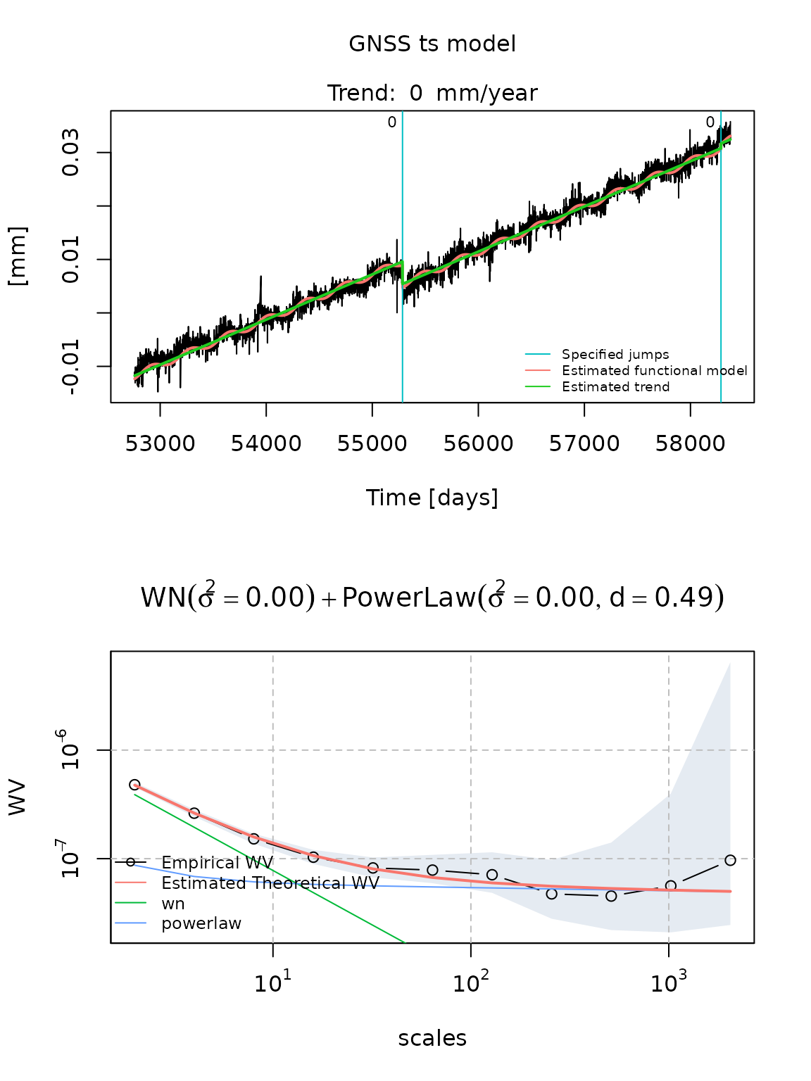

fit_dobs_wn_plp_mle$beta_hat

##          bias         trend      A*cos(U)      A*sin(U)          jump 
##  1.200000e-02  8.451006e-06 -6.672690e-04  1.359080e-06 -4.194170e-03 
##          jump 
##  9.071300e-04

fit_dobs_wn_plp_mle$theta_hat

##       wn_sigma2 powerlaw_sigma2      powerlaw_d 
##    7.779727e-07    2.700504e-07    4.854970e-01

Importing data from the Plate Boundary Observatory (PBO)

We can load time series data from the Plate Boundary Observatory (PBO) as gnssts object with PBO_get_station():

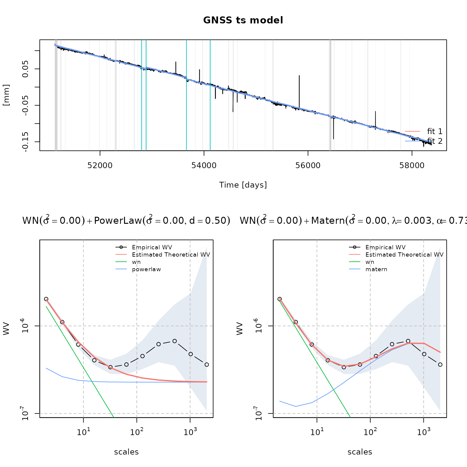
cola = PBO_get_station("COLA", column = "dE")

Comparing estimated models

Let us consider three potential models for the stochastic model of this signal. More precisely let us consider:

a White noise and a PowerLaw process
a White noise coupled with a Matérn process
a White noise and a Fractional Gaussian noise

fit_cola_wn_plp = estimate_gmwmx(cola, model_string = "wn+powerlaw", 
                                 theta_0 = c(0.1,0.1,0.1),
                                 n_seasonal = 1, 
                                 ci = T)

plot(fit_cola_wn_plp)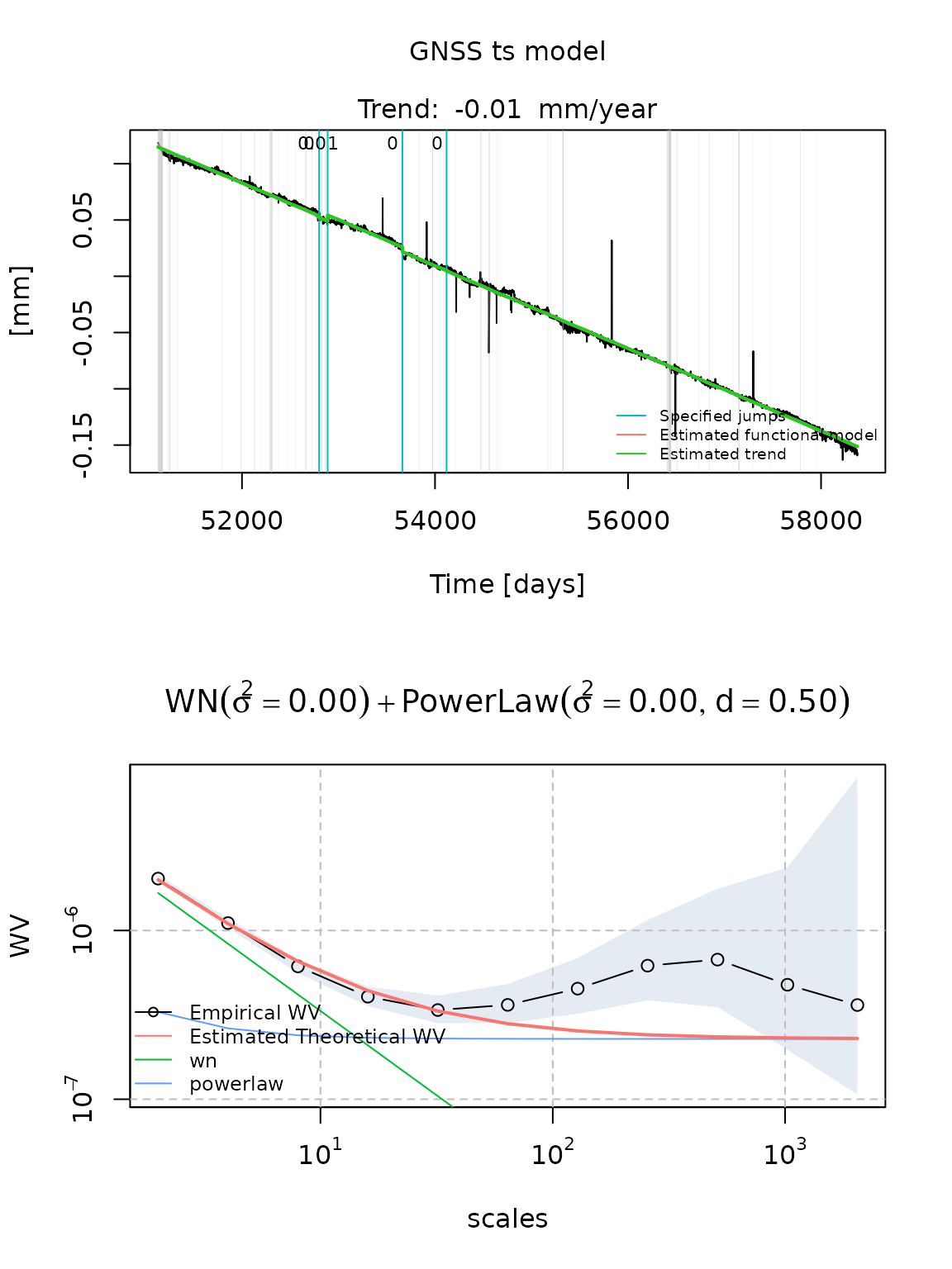

fit_cola_wn_fgn = estimate_gmwmx(cola, model_string = "wn+fgn", theta_0 = c(0.1,0.1,0.2),
                                                          n_seasonal = 1, 
                                                          ci = T)

plot(fit_cola_wn_fgn)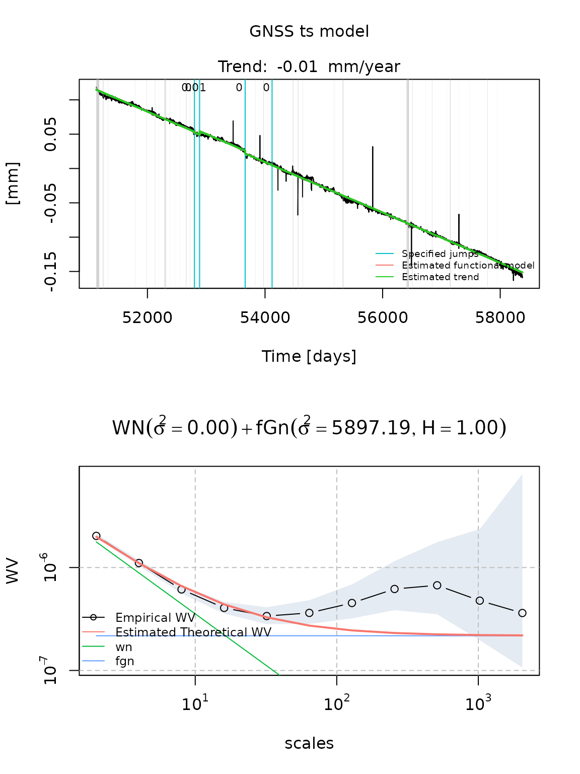

fit_cola_wn_matern = estimate_gmwmx(cola, model_string = "wn+matern", 
                                    theta_0 = c(0.1,0.1,0.1,0.1),
                                    n_seasonal = 1, 
                                    ci = T)

plot(fit_cola_wn_matern)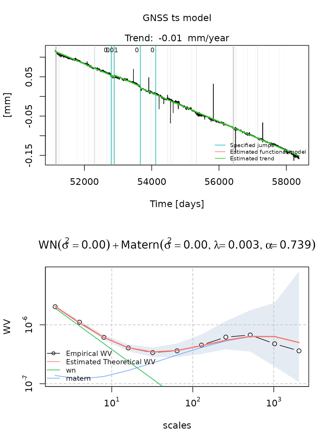

You can compare estimated models with the function compare_fits()

compare_fits(fit_cola_wn_plp, fit_cola_wn_matern)

## Warning in compare_fits(fit_cola_wn_plp, fit_cola_wn_matern): Provided fits do
## not esimate the same model.

Importing a .mom file as a gnssts object