Chapter 4 Data Structures
There are different data types that are commonly used in R among which the most important ones are the following:
Numeric (or double): these are used to store real numbers. Examples: -4, 12.4532, 6.
Integer: examples: 2L, 12L.
Logical (or boolean): examples:
TRUE,FALSE.Character: examples:
"a","Bonjour".
In R there are five types of data structures in which elements can be stored. A data structure is said to homogeneous if it only contains elements of the same type (for example it only contains character or only numeric values) and heterogenous if it contains elements of more than one type. The five types of data structures are commonly summarized in a table similar to the one below (see e.g. Wickham 2014a):
| Dimension | Homogenous | Heterogeneous |
|---|---|---|
| 1 | Vector | List |
| 2 | Matrix | Data Frame |
| n | Array |
Consider a simple data set of the top five male single tennis players presented below:
| Name | Date of Birth | Place of Birth | Place of Residence | ATP Ranking | Prize Money | Win Percentage | Grand Slam Wins | Pro Since |
|---|---|---|---|---|---|---|---|---|
| Novak Djokovic | 22 May 1987 | Belgrade, Serbia | Monte Carlo, Monaco | 1 | 135,259,120 | 82.7 | 16 | 2003 |
| Rafael Nadal | 3 June 1986 | Manacor, Spain | Manacor, Spain | 2 | 115,178,858 | 83.1 | 19 | 2001 |
| Roger Federer | 8 August 1981 | Basel, Switzerland | Wollerau, Switzerland | 3 | 126,840,700 | 82.2 | 20 | 1998 |
| Daniil Medvedev | 11 February 1996 | Moscow, Russia | Monte Carlo, Monaco | 4 | 8,171,483 | 63.6 | 0 | 2014 |
| Dominic Thiem | 3 September 1993 | Wiener Neustadt, Austria | Lichtenwörth, Austria | 5 | 18,588,662 | 64.3 | 0 | 2011 |
Notice that this data set contains a variety of data types; in the next sections we will use this data to illustrate how to work with five common data structures.
4.1 Vectors
A vector has three important properties:
- The Type of objects contained in the vector. The function
typeof()returns a description of the type of objects in a vector. - The Length of a vector indicates the number of elements in the vector. This information can be obtained using the function
length(). - Attributes are metadata attached to a vector. The functions
attr()andattributes()can be used to store and retrieve attributes (more details can be found in Section 4.1.4).
c() is a generic function that combines arguments to form a vector. All arguments are coerced to a common type (which is the type of the returned value) and all attributes except names are removed. For example, consider the number of grand slams won by the five players considered in the eighth column of Table 4.2:
To display the values stored in grand_slam_win we could simply enter the following in the R console:
## [1] 16 19 20 0 0Alternatively, we could have created and displayed the value by using () around the definition of the object itself as follows:
## [1] 16 19 20 0 0Various forms of “nested concatenation” can be used to define vectors. For example, we could also define grand_slam_win as
## [1] 16 19 20 0 0This approach is often used to assemble vectors in various ways.
It is also possible to define vectors with characters, for example we could define a vector with the player names as follows:
(players <- c("Novak Djokovic", "Rafael Nadal", "Roger Federer",
              "Daniil Medvedev", "Dominic Thiem"))
## [1] "Novak Djokovic" "Rafael Nadal" "Roger Federer" "Daniil Medvedev"
## [5] "Dominic Thiem"4.1.1 Type
We can evaluate the kind or type of elements that are stored in a vector using the function typeof(). For example, for the vectors we just created we obtain:
## [1] "double"## [1] "character"This is a little surprising since all the elements in grand_slam_win are integers and it would seem natural to expect this as an output of the function typeof(). This is because R considers any number as a “double” by default, except when adding the suffix L after an integer. For example:
## [1] "double"## [1] "integer"Therefore, we could express grand_slam_win as follows:
## [1] 16 19 20 0 0## [1] "integer"In general, the difference between the two is relatively unimportant.
4.1.2 Coercion
As indicated earlier, a vector has a homogeneous data structure meaning that it can only contain a single type among all the data types. Therefore, when more than one data type is provided, R will coerce the data into a “shared” type. To identify this “shared” type we can use this simple rule:
\[\begin{equation*} \text{logical} < \text{integer} < \text{numeric} < \text{character}, \end{equation*}\]
which simply means that if a vector has more than one data type, the “shared” type will be that of the “largest” type according to the progression shown above. For example:
## [1] 1.0 12.0 0.5## [1] "double"## [1] "14.3" "Hi"## [1] "character"4.1.3 Subsetting
Naturally, it is possible to “subset” the values of in our vector in many ways. Essentially, there are four main ways to subset a vector. Here we’ll only discuss the first three:
- Positive Index: We can access or subset the \(i\)-th element of a vector by simply using
grand_slam_win[i]where \(i\) is a positive number between 1 and the length of the vector.
## [1] 16## [1] 20 16## [1] 16 16 19 19 20 0- Negative Index: We remove elements in a vector using negative indices:
## [1] 16 20 0 0## [1] 19 20 0- Logical Indices: Another useful approach is based on logical operators:
## [1] 16 0grand_slam_win[c(-1, 2)] would produce an error message.
4.1.4 Attributes
Let’s suppose that we conduct an experiment under specific conditions, say a date and place that are stored as attributes of the object containing the results of this experiment. Indeed, objects can have arbitrary additional attributes that are used to store metadata on the object of interest. For example:
To display the vector with its attributes
## [1] 16 19 20 0 0
## attr(,"date")
## [1] "09-30-2019"
## attr(,"type")
## [1] "Men, Singles"To only display the attributes we can use
## $date
## [1] "09-30-2019"
##
## $type
## [1] "Men, Singles"It is also possible to extract a specific attribute
## [1] "09-30-2019"4.1.5 Adding Labels
In some cases, it is useful to characterize vector elements with labels. For example, we could define the vector grand_slam_win and associate the name of each corresponding athlete as a label, i.e.
(grand_slam_win <- c("Novak Djokovic" = 16, "Rafael Nadal" = 18,
"Roger Federer" = 20, "Daniil Medvedev" = 0,
"Dominic Thiem" = 0))## Novak Djokovic Rafael Nadal Roger Federer Daniil Medvedev Dominic Thiem
## 16 18 20 0 0The main advantage of this approach is that the number of grand slams won can now be referred to by the player’s name. For example:
## Novak Djokovic
## 16## Novak Djokovic Roger Federer
## 16 20All labels (athlete names in this case) can be obtained with the function names(), i.e.
## [1] "Novak Djokovic"  "Rafael Nadal"    "Roger Federer"   "Daniil Medvedev"
## [5] "Dominic Thiem"4.1.6 Working with Dates
When working with dates it is useful to treat them as real dates rather than character strings that look like dates (to a human) but don’t otherwise behave like dates. For example, consider a vector of three dates: c("03-21-2015", "12-13-2011", "06-27-2008").
The sort() function returns the elements of a vector in ascending order, but since these dates are actually just character strings that look like dates (to a human), R sorts them in alphanumeric order (for characters) rather than chronological order (for dates):
# The `sort()` function sorts elements in a vector in ascending order
sort(c("03-21-2015", "12-31-2011", "06-27-2008", "01-01-2012"))
## [1] "01-01-2012" "03-21-2015" "06-27-2008" "12-31-2011"Converting the character strings to “yyyy-mm-dd” would solve our sorting problem, but perhaps we also want to calculate the number of days between two events that are several months or years apart.
The as.Date() function is one straight-forward method for converting character strings into dates that can be used as such. The typical syntax is of the form:
Considering the dates of birth presented in Table 4.2 we can save them in an appropriate format using:
(players_dob <- as.Date(c("22 May 1987", "3 Jun 1986", "8 Aug 1981",
                         "11 Feb 1996", "3 Sep 1993"),
                       format = "%d %b %Y"))
## [1] "1987-05-22" "1986-06-03" "1981-08-08" "1996-02-11" "1993-09-03"Note the syntax of format = "%d %b %Y". The following table shows common format elements for use with the as.Date() function:
| Symbol | Meaning | Example |
|---|---|---|
| %d | day as a number (0-31) | 01-31 |
| %a | abbreviated weekday | Mon |
| %A | unabbreviated weekday | Monday |
| %m | month (00-12) | 00-12 |
| %b | abbreviated month | Jan |
| %B | unabbreviated month | January |
| %y | 2-digit year | 07 |
| %Y | 4-digit year | 2007 |
There are many advantages to using the as.Date() format (in addition to proper sorting). For example, the subtraction between two dates becomes more meaningful and yields the difference in days between them. As an example, the number of days between Rafael Nadal’s and Andy Murray’s dates of birth can be obtained as
## Time difference of 353 daysIn addition, subsetting becomes also more intuitive and, for example, to find the players born after 1 January 1986 we can simply run:
## [1] "Novak Djokovic" "Rafael Nadal" "Daniil Medvedev" "Dominic Thiem"There are many other reasons for using this format (or other date formats). A more detailed discussion on this topic can, for example, be found in Cole Beck’s notes.
4.1.7 Useful Functions with Vectors
The reason for extracting or creating vectors often lies in the need to collect information from them. For this purpose, a series of useful functions are available that allow to extract information or arrange the vector elements in a certain way which can be of interest to the user. Among the most commonly used functions we can find the following ones
length() sum() mean() order() and sort()
whose name is self-explanatory in most cases. For example we have
## [1] 5## [1] 54## [1] 10.8To sort the players by number of grand slam wins, we could use the function order() which returns the position of the elements of a vector sorted in an ascending order,
## [1] 4 5 1 2 3Therefore, we can sort the players in ascending order of wins as follows
## [1] "Daniil Medvedev" "Dominic Thiem"   "Novak Djokovic"  "Rafael Nadal"
## [5] "Roger Federer"
which implies that Roger Federer won most grand slams. Another related function is sort() which simply sorts the elements of a vector in an ascending manner. For example,
## Daniil Medvedev   Dominic Thiem  Novak Djokovic    Rafael Nadal   Roger Federer
##               0               0              16              18              20
which is compact version of
## Daniil Medvedev   Dominic Thiem  Novak Djokovic    Rafael Nadal   Roger Federer
##               0               0              16              18              20
It is also possible to use the functions sort() and order() with characters and dates. For example, to sort the players’ names alphabetically (by first name) we can use:
## [1] "Daniil Medvedev" "Dominic Thiem"   "Novak Djokovic"  "Rafael Nadal"
## [5] "Roger Federer"
Similarly, we can sort players by age (oldest first)
## [1] "Roger Federer"   "Rafael Nadal"    "Novak Djokovic"  "Dominic Thiem"
## [5] "Daniil Medvedev"
or in an reversed manner (oldest last):
## [1] "Daniil Medvedev" "Dominic Thiem"   "Novak Djokovic"  "Rafael Nadal"
## [5] "Roger Federer"
There are of course many other useful functions that allow to deal with vectors which we will not mention in this section but can be found in a variety of references (see e.g. Wickham 2014a).
4.1.8 Creating sequences
When using R for statistical programming and data analysis it is very common to create sequences of numbers. Here are three common ways used to create such sequences:
from:to: This method is quite intuitive and very compact. For example:
## [1] 1 2 3## [1] 3 2 1## [1] -1 -2 -3 -4## [1] 1.3 2.3seq_len(n): This function provides a simple way to generate a sequence from 1 to an arbitrary numbern. In general,1:nandseq_len(n)are equivalent with the notable exceptions wheren = 0andn < 0. The reason for these exceptions will become clear in Section 5.2.3.1. Let’s see a few examples:
## [1] 1 2 3## [1] 1 2 3## [1] 1 0## integer(0)seq(a, b, by/length.out = d): This function can be used to create more “complex” sequences. It can either be used to create a sequence fromatobby increments ofd(using the optionby) or of a total length ofd(using the optionlength.out). A few examples:
## [1] 1.0 1.4 1.8 2.2 2.6## [1] 1.00 1.36 1.72 2.08 2.44 2.80This can be combined with the rep() function to create vectors with repeated values or sequences, for example:
## [1] 1 2 1 2 1 2## [1] 1 1 1 2 2 2## [1] 1 1 2 2 1 1 2 2where the option times allows to specify how many times the object needs to be repeated and each regulates how many times each element in the object is repeated.
It is also possible to generate sequences of dates using the function seq(). For example, to generate a sequence of 10 dates between the dates of birth of Andy Murray and Rafael Nadal we can use
##  [1] "1987-05-22" "1987-04-12" "1987-03-04" "1987-01-24" "1986-12-16"
##  [6] "1986-11-06" "1986-09-28" "1986-08-20" "1986-07-12" "1986-06-03"
Similarly, we can create a sequence between the two dates by increments of one week (backwards)
##  [1] "1987-05-22" "1987-05-15" "1987-05-08" "1987-05-01" "1987-04-24"
##  [6] "1987-04-17" "1987-04-10" "1987-04-03" "1987-03-27" "1987-03-20"
## [11] "1987-03-13" "1987-03-06" "1987-02-27" "1987-02-20" "1987-02-13"
## [16] "1987-02-06" "1987-01-30" "1987-01-23" "1987-01-16" "1987-01-09"
## [21] "1987-01-02" "1986-12-26" "1986-12-19" "1986-12-12" "1986-12-05"
## [26] "1986-11-28" "1986-11-21" "1986-11-14" "1986-11-07" "1986-10-31"
## [31] "1986-10-24" "1986-10-17" "1986-10-10" "1986-10-03" "1986-09-26"
## [36] "1986-09-19" "1986-09-12" "1986-09-05" "1986-08-29" "1986-08-22"
## [41] "1986-08-15" "1986-08-08" "1986-08-01" "1986-07-25" "1986-07-18"
## [46] "1986-07-11" "1986-07-04" "1986-06-27" "1986-06-20" "1986-06-13"
## [51] "1986-06-06"
or by increments of one month (forwards)
##  [1] "1986-06-03" "1986-07-03" "1986-08-03" "1986-09-03" "1986-10-03"
##  [6] "1986-11-03" "1986-12-03" "1987-01-03" "1987-02-03" "1987-03-03"
## [11] "1987-04-03" "1987-05-03"
4.1.9 Example: Apple Stock Price
Suppose that someone is interested in analyzing the behavior of Apple’s stock price over the last three months. The first thing needed to perform such analysis is to recover (automatically) today’s date. In R, this can be obtained as follows
## [1] "2019-04-18"Once this is done, we can obtain the date which is exactly three months ago by using
## [1] "2019-01-18"With this information, we can now download Apple’s stock price and represent these stocks through a candlestick chart which summarizes information on daily opening and closing prices as well as minimum and maximum prices. These charts are often used with the hope of detecting trading patterns over a given period of time.
library(quantmod)
getSymbols("AAPL", from = three_months_ago, to = today)
candleChart(AAPL, theme = 'white', type = 'candles')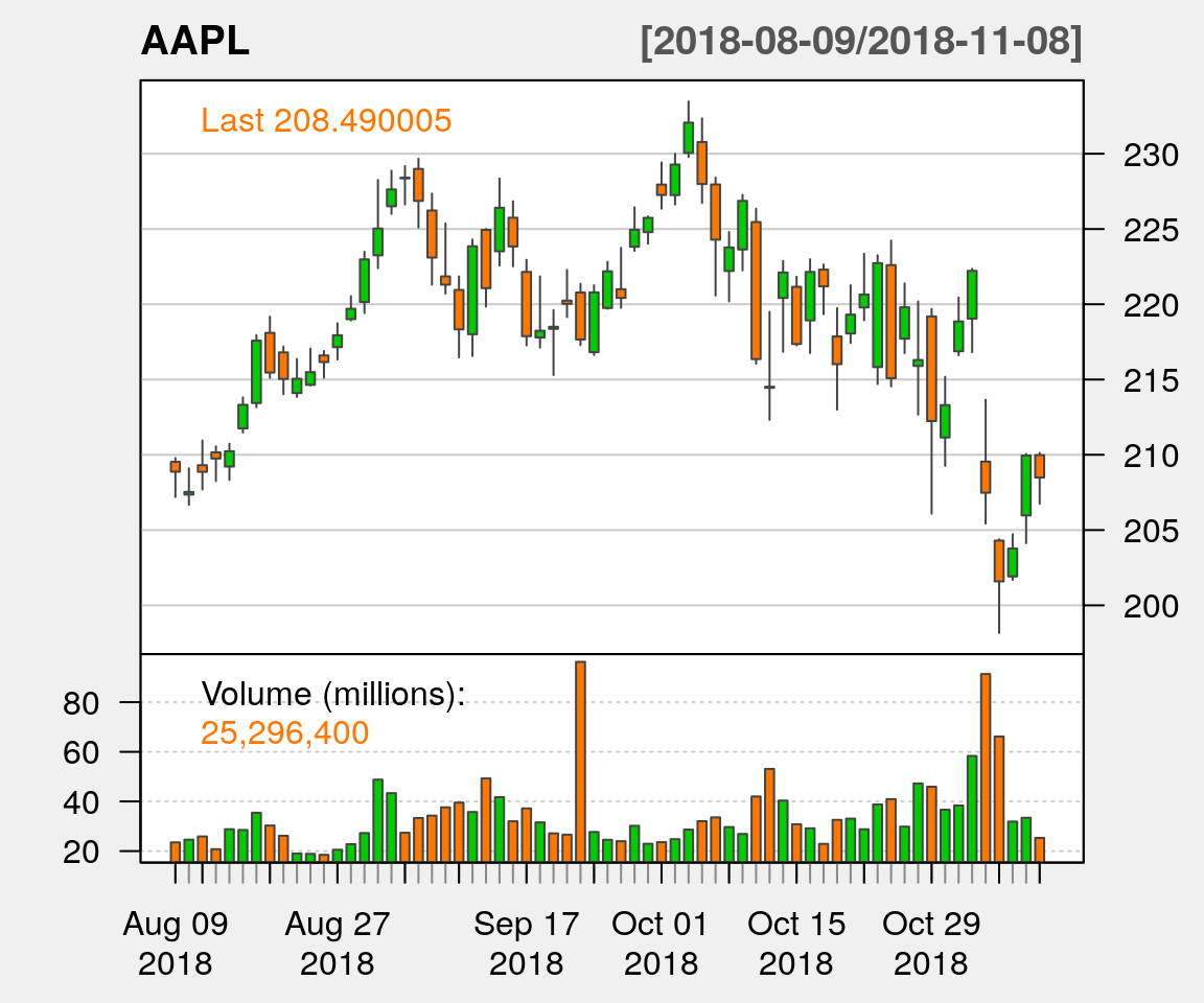
Figure 4.1: Candlestick chart for Apple’s stock price for the last three months.
Using the price contained in the object we downloaded (i.e. AAPL), we can compute Apple’s arithmetic returns which are defined as follows
\[\begin{equation} R_t = \frac{S_t - S_{t-1}}{S_{t-1}}, \tag{4.1} \end{equation}\]
where \(R_t\) are the returns at time t and \(S_t\) is the stock price. This is implemented in the function ClCl() within the quantmod package. For example, we can create a vector of returns as follows
where na.omit() is used to remove missing values in the stock prices vector since, if we have \(n+1\) stock prices, we will only have \(n\) returns and therefore the first return cannot be computed. We can now compute the mean and median of the returns over the considered period.
## [1] 0.0001369265## [1] 0.003158065However, a statistic that is of particular interest to financial operators is the Excess Kurtosis which, for a random variable that we denote as \(X\), can be defined as
\[\begin{equation} \text{Kurt} = \frac{{\mathbb{E}}\left[\left(X - \mathbb{E}[X]\right)^4\right]}{\left({\mathbb{E}}\left[\left(X - \mathbb{E}[X]\right)^2\right]\right)^2} - 3. \end{equation}\]
The reason for defining this statistic as Excess Kurtosis lies in the fact that the standardized kurtosis is compared to that of a Gaussian distribution (whose kurtosis is equal to 3) which has exponentially decaying tails. Consequently, if the Excess Kurtosis is positive, this implies that the distribution has heavier tails than a Gaussian and therefore has higher probabilities of extreme events occurring. To understand why the Excess Kurtosis is equal to 0 for a Gaussian distribution click on the button below:
Assuming \(X\) to be Gaussian, we have \(X \sim \mathcal{N}(\mu, \sigma^2)\). Then, we define \(Z\) as \(Z \sim \mathcal{N}(0,1)\) and \(Y\) as \(Y = Z^2 \sim \chi^2_1\). Remember that a random variable following a \(\chi^2_1\) distribution has the following properties: \(\text{Var}[Y] = 2\) and \(\mathbb{E}[Y] = 1\). Using these definitions and properties, we obtain:
\[\begin{equation} \begin{aligned} \text{Kurt} &= \frac{{\mathbb{E}}\left[\left(X - \mathbb{E}[X]\right)^4\right]}{\left({\mathbb{E}}\left[\left(X - \mathbb{E}[X]\right)^2\right]\right)^2} - 3 = \frac{{\mathbb{E}}\left[\left(X - \mathbb{E}[X]\right)^4\right]}{\left[\text{Var} \left(X\right)\right]^2} - 3 = \frac{{\mathbb{E}}\left[\left(X - \mathbb{E}[X]\right)^4\right]}{\sigma^4} - 3\\ &= {\mathbb{E}}\left[\left(\frac{X - \mathbb{E}[X]}{\sigma}\right)^4\right] - 3 = \mathbb{E}\left[Z^4\right] - 3 = \text{Var}[Z^2] + \mathbb{E}^2\left[Z^2\right] - 3\\ &= \text{Var}[Y] + \mathbb{E}^2\left[Y\right] - 3 = 0. \end{aligned} \end{equation}\]
This implies that the theoretical value of the excess Kurtosis for a normally distributed random variable is \(0\).Given this statistic, it is useful to compute this on the observed data and for this purpose a common estimator of the excess Kurtosis is
\[\begin{equation} k = \frac{\frac{1}{n} \sum_{t = 1}^{n} \left(R_t -\bar{R}\right)^4}{\left(\frac{1}{n} \sum_{t = 1}^{n} \left(R_t -\bar{R}\right)^2 \right)^2} - 3, \end{equation}\]
where \(\bar{R}\) denotes the sample average of the returns, i.e.
\[\begin{equation*} \bar{R} = \frac{1}{n} \sum_{i = 1}^n R_i. \end{equation*}\]
In R, this can simply be done as follows:
## [1] 1.724814Therefore, we observe an estimated Excess Kurtosis of 1.72 which is quite high and tends to indicate that the returns have heavier tails than the normal distribution. In Chapter 5, we will revisit this example and investigate if there is enough evidence to conclude that Apple’s stock has Excess Kurtosis larger than zero.
4.2 Matrices
Matrices are a common data structure in R which have two dimensions to store multiple vectors of the same length combined as a unified object. The matrix() function can be used to create a matrix from a vector:
##      [,1] [,2] [,3] [,4]
## [1,]    1    4    7   10
## [2,]    2    5    8   11
## [3,]    3    6    9   12
Notice that the first argument to the function is a vector (in this case the sequence 1 to 12) which is then transformed into a matrix with four columns (ncol = 4) and three rows (nrow = 3).
By default, the vectors are transformed into matrices by placing the elements by column (i.e. top to the bottom of ech column in sequence until all columns are full). If you wish to fill the matrix by row, all you need to do is specify the argument byrow = T.
##      [,1] [,2] [,3] [,4]
## [1,]    1    2    3    4
## [2,]    5    6    7    8
## [3,] 9 10 11 12It is often the case that we already have equi-dimensional vectors available and we wish to bundle them together as matrix. In these cases, two useful functions are cbind() to combine vectors as vertical columns side-by-side, and rbind() to combine vectors as horizontal rows. An example of cbind() is shown here:
players <- c("Novak Djokovic", "Rafael Nadal", "Roger Federer",
             "Daniil Medvedev", "Dominic Thiem")
grand_slam_win <- c(16, 19, 20, 0, 0)
win_percentage <- c(82.7, 83.1, 82.2, 63.6, 64.3)
(mat <- cbind(grand_slam_win, win_percentage))
## grand_slam_win win_percentage
## [1,] 16 82.7
## [2,] 19 83.1
## [3,] 20 82.2
## [4,] 0 63.6
## [5,] 0 64.3The result in this case is a \(5 \times 2\) matrix (with rbind() it would have been a \(2 \times 5\) matrix). Once the matrix is defined, we can assign names to its rows and columns by using rownames() and colnames(), respectively. Of course, the number of names must match the corresponding matrix dimension. In the following example, each row corresponds to a specific player (thereby using the players vector) and each column corresponds to a specific statistic of the players.
## GS win Win rate
## Novak Djokovic 16 82.7
## Rafael Nadal 19 83.1
## Roger Federer 20 82.2
## Daniil Medvedev 0 63.6
## Dominic Thiem 0 64.34.2.1 Subsetting
As with vectors, it is possible to subset the elements of a matrix. Since matrices are two-dimensional data structures, it is necessary to specify the position of the elements of interest in both dimensions. For this purpose we can use [ , ] immediately following the named matrix. Note the use of , within the square brackets in order to specify both row and column position of desired elements within the matrix (e.g. matrixName[row, column]). Consider the following examples:
# Subset players "Dominic Thiem" and "Roger Federer" in matrix named "mat"
mat[c("Dominic Thiem", "Roger Federer"), ]## GS win Win rate
## Dominic Thiem 0 64.3
## Roger Federer 20 82.2## GS win Win rate
## Novak Djokovic 16 82.7
## Roger Federer 20 82.2## Novak Djokovic Rafael Nadal Roger Federer Daniil Medvedev Dominic Thiem
## 82.7 83.1 82.2 63.6 64.3## Novak Djokovic Rafael Nadal Roger Federer
## 16 19 20It can be noticed that, when a space is left blank before or after the comma, this means that respectively all the rows or all the columns are considered.
4.2.2 Matrix Operators in R
As with vectors, there are some useful functions that can be used with matrices. A first example is the function dim() that allows to determine the dimension of a matrix. For example, consider the following \(4 \times 2\) matrix
\[\begin{equation*} \mathbf{A} = \left[ \begin{matrix} 1 & 5\\ 2 & 6\\ 3 & 7\\ 4 & 8 \end{matrix} \right] \end{equation*}\]
which can be created in R as follows:
## [,1] [,2]
## [1,] 1 5
## [2,] 2 6
## [3,] 3 7
## [4,] 4 8Therefore, we expect dim(A) to return the vector c(4, 2). Indeed, we have
## [1] 4 2Next, we consider the function t() that allows transpose a matrix. For example, \(\mathbf{A}^T\) is equal to:
\[\begin{equation*} \mathbf{A}^T = \left[ \begin{matrix} 1 & 2 & 3 & 4\\ 5 & 6 & 7 & 8 \end{matrix} \right], \end{equation*}\]
which is a \(2 \times 4\) matrix. In R, we achieve this as follows
## [,1] [,2] [,3] [,4]
## [1,] 1 2 3 4
## [2,] 5 6 7 8## [1] 2 4Aside from playing with matrix dimensions, matrix algebraic operations have specific commands. For example, the operator %*% is used in R to denote matrix multiplication while, as opposed to scalar objects, the regular product operator * performs the element by element product (or Hadamard product) when applied to matrices. For example, consider the following matrix product:
\[\begin{equation*} \mathbf{B} = \mathbf{A}^T \mathbf{A} = \left[ \begin{matrix} 30 & 70\\ 70 & 174 \end{matrix} \right], \end{equation*}\]
which can be done in R as follows:
## [,1] [,2]
## [1,] 30 70
## [2,] 70 174Other common matrix operations include finding the determinant of a matrix and finding its inverse. These are often used, for example, when computing the likelihood function for a variable following a Gaussian distribution or when simulating time series or spatial data. The functions that perform these operations are det() and solve() that respectively find the determinant and the inverse of a matrix (which necessarily has to be square). The function det() can be used to compute the determinant of a square matrix. In the case of a \(2 \times 2\) matrix, there exists a simple solution for the determinant which is
\[\begin{equation*} \text{det} \left( \mathbf{D} \right) = \text{det} \left( \left[ \begin{matrix} d_1 & d_2\\ d_3 & d_4 \end{matrix} \right] \right) = d_1 d_4 - d_2 d_3. \end{equation*}\]
Consider the matrix \(\mathbf{B}\), we have
\[\begin{equation*} \text{det} \left( \mathbf{B}\right) = 30 \cdot 174 - 70^2 = 320. \end{equation*}\]
In R, we can simply do
## [1] 320The function solve() is also an important function when working with matrices as it allows to inverse a matrix. It is worth remembering that a square matrix that is not invertible (i.e. \(\mathbf{A}^{-1}\) doesn’t exist) is called singular and the determinant offers a way to “check” if this is the case for a given matrix. Indeed, a square matrix is singular if and only if its determinant is 0. Therefore, in the case of \(\mathbf{B}\), we should be able to compute its inverse. As for the determinant, there exists a formula to compute the inverse of \(2 \times 2\) matrices, i.e.
\[\begin{equation*} \mathbf{D}^{-1} = \left[ \begin{matrix} d_1 & d_2\\ d_3 & d_4 \end{matrix} \right]^{-1} = \frac{1}{\text{det}\left( \mathbf{D} \right)} \left[ \begin{matrix} \phantom{-}d_4 & -d_2\\ -d_3 & \phantom{-}d_1 \end{matrix} \right]. \end{equation*}\]
Considering the matrix \(\mathbf{B}\), we obtain
\[\begin{equation*} \mathbf{B}^{-1} = \left[ \begin{matrix} 30 & 70\\ 70 & 174 \end{matrix} \right]^{-1} = \frac{1}{320}\left[ \begin{matrix} \phantom{-}174 & -70\\ -70 & \phantom{-}30 \end{matrix} \right] = \left[ \begin{matrix} \phantom{-}0.54375 & -0.21875\\ -0.21875 & \phantom{-}0.09375 \end{matrix} \right] \end{equation*}\]
## [,1] [,2]
## [1,] 0.54375 -0.21875
## [2,] -0.21875 0.09375Finally, we can verify that
\[\begin{equation*} \mathbf{G} = \mathbf{B} \mathbf{B}^{-1}, \end{equation*}\]
should be equal to the identity matrix,
## [,1] [,2]
## [1,] 1 -8.881784e-16
## [2,] 0 1.000000e+00The result is of course extremely close but \(\mathbf{G}\) is not exactly equal to the identity matrix due to rounding and other numerical errors.
Another function of interest is the function diag() that can be used to extract the diagonal of a matrix. For example, we have
\[\begin{equation*} \text{diag} \left( \mathbf{B} \right) = \left[30 \;\; 174\right], \end{equation*}\]
which can be done in R as follows:
## [1] 30 174Therefore, the function diag() computes the trace of matrix (i.e. the sum of the diagonal elements). For example,
\[\begin{equation*} \text{tr} \left( \mathbf{B} \right) = 204, \end{equation*}\]
or in R:
## [1] 204Another use of the function diag() is to create diagonal matrices. Indeed, if the argument of this function is a vector, its behavior is the following:
\[\begin{equation*} \text{diag} \left(\left[a_1 \;\; a_2 \;\; \cdots \;\; a_n\right]\right) = \left[ \begin{matrix} a_1 & 0 & \cdots & 0 \\ 0 & a_2 & \cdots & 0 \\ \vdots & \vdots & \ddots & \vdots \\ 0 & 0 & \cdots & a_n \end{matrix} \right]. \end{equation*}\]
Therefore, this provides a simple way of creating an identity matrix by combining the functions diag() and rep() (discussed in the previous section) as follows:
## [,1] [,2] [,3] [,4]
## [1,] 1 0 0 0
## [2,] 0 1 0 0
## [3,] 0 0 1 0
## [4,] 0 0 0 14.2.3 Example: Summary Statistics with Matrix Notation
A simple example of the operations we discussed in the previous section is given by many common statistics that can be re-expressed using matrix notation. As an example, we will consider three common statistics that are the sample mean, variance and covariance. Let us consider the following two samples of size \(n\)
\[\begin{equation*} \begin{aligned} \mathbf{x} &= \left[x_1 \;\; x_2 \; \;\cdots \;\; x_n\right]^T\\ \mathbf{y} &= \left[y_1 \;\;\; y_2 \; \;\;\cdots \;\;\; y_n\right]^T. \end{aligned} \end{equation*}\]
The sample mean of \(\mathbf{x}\) is
\[\begin{equation*} \bar{x} = \frac{1}{n} \sum_{i = 1}^{n} x_i, \end{equation*}\]
and its sample variance is
\[\begin{equation*} s_x^2 = \frac{1}{n} \sum_{i = 1}^n \left(x_i - \bar{x}\right)^2. \end{equation*}\]
The sample covariance between \(\mathbf{x}\) and \(\mathbf{y}\) is
\[\begin{equation*} s_{x,y} = \frac{1}{n} \sum_{i = 1}^n \left(X_i - \bar{x}\right) \left(Y_i - \bar{y}\right), \end{equation*}\]
where \(\bar{y}\) denotes the sample mean of \(\mathbf{y}\).
Consider the sample mean, this statistic can be expressed in matrix notation as follows
\[\begin{equation*} \bar{x} = \frac{1}{n} \sum_{i = 1}^{n} x_i = \frac{1}{n} \mathbf{x}^T \mathbf{1}, \end{equation*}\]
where \(\mathbf{1}\) is a column vector of \(n\) ones.
\[\begin{equation*} \begin{aligned} s_x^2 &= \frac{1}{n} \sum_{i = 1}^n \left(x_i - \bar{x}\right)^2 = \frac{1}{n} \sum_{i = 1}^n x_i^2 - \bar{x}^2 = \frac{1}{n} \mathbf{x}^T \mathbf{x} - \bar{x}^2\\ &= \frac{1}{n} \mathbf{x}^T \mathbf{x} - \left(\frac{1}{n} \mathbf{x}^T \mathbf{1}\right)^2 = \frac{1}{n} \left(\mathbf{x}^T \mathbf{x} - \frac{1}{n} \mathbf{x}^T \mathbf{1} \mathbf{1}^T \mathbf{x}\right)\\ &= \frac{1}{n}\mathbf{x}^T \left( \mathbf{I} - \frac{1}{n} \mathbf{1} \mathbf{1}^T \right) \mathbf{x} = \frac{1}{n}\mathbf{x}^T \mathbf{H} \mathbf{x}, \end{aligned} \end{equation*}\]
where \(\mathbf{H} = \mathbf{I} - \frac{1}{n} \mathbf{1} \mathbf{1}^T\). This matrix is often called the centering matrix. Similarly, for the sample covariance we obtain
\[\begin{equation*} \begin{aligned} s_{x,y} &= \frac{1}{n} \sum_{i = 1}^n \left(x_i - \bar{x}\right) \left(y_i - \bar{y}\right) = \frac{1}{n}\mathbf{x}^T \mathbf{H} \mathbf{y}. \end{aligned} \end{equation*}\]
In the code below we verify the validity of these results through a simple simulated example where we compare the values of the three statistics based on the different formulas discussed above.
# Sample size
n <- 100
# Simulate random numbers from a zero mean normal distribution with
# variance equal to 4.
x <- rnorm(n, 0, sqrt(4))
# Simulate random numbers from normal distribution with mean 3 and
# variance equal to 1.
y <- rnorm(n, 3, 1)
# Note that x and y are independent.
# Sample mean
one <- rep(1, n)
x_bar <- 1/n*sum(x)
x_bar_mat <- 1/n*t(x)%*%one
# Sample variance of x
H <- diag(rep(1, n)) - 1/n * one %*% t(one)
s_x <- 1/n * sum((x - x_bar)^2)
s_x_mat <- 1/n*t(x) %*% H %*% x
# Sample covariance
y_bar <- 1/n*sum(y)
s_xy <- 1/n*sum((x - x_bar)*(y - y_bar))
s_xy_mat <- 1/n*t(x) %*% H %*% yTo compare, let’s construct a matrix of all the results that we calculated.
cp_matrix <- matrix(c(x_bar, x_bar_mat, s_x, s_x_mat, s_xy, s_xy_mat), ncol = 2, byrow = T)
row.names(cp_matrix) <- c("Sample Mean", "Sample Variance", "Sample Covariance")
colnames(cp_matrix) <- c("Scalar", "Matrix")
cp_matrix## Scalar Matrix
## Sample Mean -0.095715724 -0.095715724
## Sample Variance 3.485078494 3.485078494
## Sample Covariance -0.007969419 -0.007969419Therefore, using the previously obtained results we can construct the following empirical covariance matrix
\[\begin{equation} \widehat{\text{Cov}}(X, Y) = \left[ \begin{matrix} s_x^2 & s_{x,y} \\ s_{x,y} & s_y^2 \end{matrix} \right]. \end{equation}\]
In R, this can be done as
# Sample variance of y
s_y_mat <- 1/n*t(y) %*% H %*% y
# Covariance matrix
(V <- matrix(c(s_x_mat, s_xy_mat, s_xy_mat, s_y_mat), 2, 2))## [,1] [,2]
## [1,] 3.485078494 -0.007969419
## [2,] -0.007969419 0.956116661This result can now be compared to
## x y
## x 3.520281307 -0.008049918
## y -0.008049918 0.965774405We can see that the results are slightly different from what we expected. This is because the calculation of cov() within the default R stats package is based on an unbiased estimator which is not the one we used. To obtain the same result, we can go back to our estimation by calculating via the below method
## x y
## x 3.485078494 -0.007969419
## y -0.007969419 0.9561166614.2.4 Example: Portfolio Optimization
Suppose that you are interested in investing your money in two stocks, say Apple and Netflix. However, you are wondering how much of each stock you should buy. To make it simple let us assume that you will invest \(\omega W\) in Apple (AAPL) and \((1-\omega) W\) in Netflix (NFLX), where \(W\) denotes the amount of money you would like to invest, and \(\omega \in [0, \, 1]\) dictates the proportion allocated to each investment. Let \(R_A\) and \(R_N\) denote, respectively, the daily return (see Equation (4.1) if you don’t remember what returns are) of Apple and Netflix. To make things simple we assume that the returns \(R_A\) and \(R_N\) are jointly normally distributed so we can write
\[ \mathbf{R} \stackrel{iid}{\sim} \mathcal{N} \left(\boldsymbol{\mu}, \boldsymbol{\Sigma}\right), \]
where
\[ \mathbf{R} = \left[ \begin{matrix} R_A\\ R_N \end{matrix} \right], \;\;\;\; \boldsymbol{\mu} = \left[ \begin{matrix} \mu_A\\ \mu_N \end{matrix} \right], \;\; \text{and}\;\; \boldsymbol{\Sigma} = \left[ \begin{matrix} \sigma_A^2 & \sigma_{AN}\\ \sigma_{AN} & \sigma_N^2 \end{matrix} \right]. \]
Using these assumptions, the classical portfolio optimization problem, which would allow you to determine a “good” value of \(\omega\), can be stated as follows: Given our initial wealth \(W\), the investment problem is to decide how much should be invested in our first asset (Apple) and in our second asset (Netflix). As mentioned earlier, we assume that \(\omega \in [0,\,1]\), implying that it is only possible to buy the two assets (i.e. short positions are not allowed). Therefore, to solve our investment problem we must choose the value of \(\omega\) which would maximize your personal utility. Informally speaking, the utility represents a measurement of the “usefulness” that is obtained from your investment. To consider a simple case, we will assume that you are a particularly risk averse individual (i.e. you are looking for an investment that is as sure and safe as possible) and as such you want to pick the value of \(\omega\) providing you with the smallest investment risk. We can then determine the optimal value of \(\omega\) as follows. First, we construct a new random variable, say \(Y\), which denotes the return of your portfolio. Since you invest \(\omega W\) in Apple and \((1 - \omega) W\) in Netflix, it is easy to see that
\[Y = \left[\omega R_A + (1 - \omega) R_N \right]W.\]
In general the risk and variance of an investment are two different things but in our case we assume that the return \(\mathbf{R}\) is normally distributed and in this case the variance can perfectly characterize the risk of our investment. Therefore, we can define the risk of our investment as the following function of \(\omega\)
\[f(\omega) = \text{Risk}(Y) = \text{Var} (Y) = \left[\omega^2 \sigma_A^2 + (1 - \omega)^2 \sigma_N^2 + 2 \omega (1 - \omega) \sigma_{AN}\right]W^2.\]
The function \(f(\omega)\) is minimized for the value \(\omega^*\) which is given by
\[\begin{equation} \omega^* = \frac{\sigma^2_N - \sigma_{AN}}{\sigma^2_A + \sigma^2_N - 2\sigma_{AN}}. \tag{4.2} \end{equation}\]
If you are interested in understanding how Equation (4.2) was obtained, click on the button below:
To obtain \(\omega^*\) we first differentiate the function \(f(\omega)\) with respect to \(\omega\), which gives
\[\begin{equation} \frac{\partial}{\partial \omega} \, f(\omega) = \left[2 \omega \sigma_A^2 - 2 (1 - \omega) \sigma_N^2 + 2 (1 - 2\omega) \sigma_{AN}\right]W^2 \end{equation}\]
Then, we define \(\omega^*\) as
\[\begin{equation} \omega^* \; : \frac{\partial}{\partial \omega} \, f(\omega) = 0. \end{equation}\]
Therefore, we obtain
\[\begin{equation} \omega^* \left(\sigma_A^2 + \sigma_N^2 - 2 \sigma_{AN}\right) = \sigma_N^2 - \sigma_{AN}, \end{equation}\]
which simplifies to
\[\begin{equation} \omega^* = \frac{\sigma_N^2 - \sigma_{AN}}{\sigma_A^2 + \sigma_N^2 - 2 \sigma_{AN}}. \end{equation}\]
Finally, we verify that our result is a minimum by considering the second derivative, i.e.
\[\begin{equation} \frac{\partial^2}{\partial \omega^2} \, f(\omega) = 2W\left[\sigma_A^2 + \sigma_N^2 - 2\sigma_{AN} \sigma_{AN}\right]. \end{equation}\]
Since \(W\) is strictly positive, all that remains to conclude our derivation is to verify that \(\sigma_A^2 + \sigma_N^2 - 2\sigma_{AN} \sigma_{AN} \leq 0\). In fact, this is a well known inequality which is a direct consequence of the Tchebychev inequality. However, here is a simpler argument to understand why this is the case. Indeed, it is obvious that \(\text{Var}(R_A - R_N) \leq 0\) and we also have \(\text{Var}(R_A - R_N) = \sigma_A^2 + \sigma_N^2 - 2\sigma_{AN}\). Thus, we obtain
\[\text{Var}(R_A - R_N) = \sigma_A^2 + \sigma_N^2 - 2\sigma_{AN} \leq 0,\]
which verifies that our result is a minimum.Using (4.2), we obtain that the expected value and variance of our investment are given by
\[ \begin{aligned} \text{Expected Value Investment} &=\left[\omega^* \mu_A + (1 - \omega^*) \mu_N\right] W,\\ \text{Variance Investment} &= \left[(\omega^*)^2 \sigma_A^2 + (1 - \omega^*)^2 \sigma_N^2 + 2 \omega^* (1 - \omega^*) \sigma_{AN}\right]W^2. \end{aligned} \]
In practice, the vector \(\boldsymbol{\mu}\) and the matrix \(\boldsymbol{\Sigma}\) are unknown and must be estimated using historical data. In the code below, we compute the optimal value of \(\omega\) based on (4.2) by using the last five years of historical data for the two stocks considered. For simplicity we set \(W\) to one but note that \(W\) plays no role in determining \(\omega^*\).
# Load quantmod
library(quantmod)
# Download data
today <- Sys.Date()
five_years_ago <- seq(today, length = 2, by = "-5 year")[2]
getSymbols("AAPL", from = five_years_ago, to = today)
getSymbols("NFLX", from = five_years_ago, to = today)
# Compute returns
Ra <- na.omit(ClCl(AAPL))
Rn <- na.omit(ClCl(NFLX))
# Estimation of mu and Sigma
Sigma <- cov(cbind(Ra, Rn))
mu <- c(mean(Ra), mean(Rn))
# Compute omega^*
omega_star <- (Sigma[2, 2] - Sigma[1, 2])/(Sigma[1, 1] + Sigma[2, 2] - 2*Sigma[1, 2])
# Compute investment expected value and variance
mu_investment <- omega_star*mu[1] + (1 - omega_star)*mu[2]
var_investment <- omega_star^2*Sigma[1,1] + (1 - omega_star)^2*Sigma[2,2] +
2*omega_star*(1 - omega_star)*Sigma[1,2]From this code, we obtain \(\omega^* \approx\) 86.03%. In the table below we compare the empirical expected values and variances of the stocks as well as those of our investment:
investment_summary <- matrix(NA, 2, 3)
dimnames(investment_summary)[[1]] <- c("Expected value", "Variance")
dimnames(investment_summary)[[2]] <- c("Apple", "Netflix", "Investment")
investment_summary[1, ] <- c(mu, mu_investment)
investment_summary[2, ] <- c(diag(Sigma), var_investment)
knitr::kable(investment_summary)| Apple | Netflix | Investment | |
|---|---|---|---|
| Expected value | 0.0009275 | 0.0018499 | 0.0010563 |
| Variance | 0.0002109 | 0.0007084 | 0.0001975 |
In Table 4.4 and the plot below we can observe that Netflix has high risk and high return. Apple seems like a safer investment in terms of risk but lower in expected return. Our portfolio optimization investment, however, seems to be in a good area, meaning that it has low risk and a return that is between the two stocks mentioned above. Finally, we provide a graphical representation of the obtained results in the figure below.
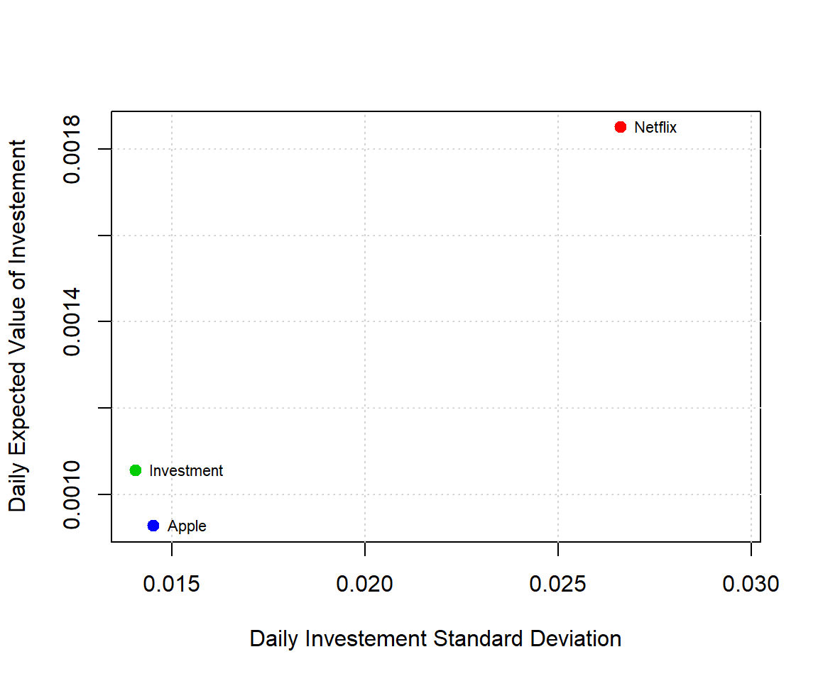
Figure 4.2: Graphical representation of Apple, Netflix and min-variance portfolio based on these two assets.
4.3 Array
Arrays allow to construct multidimensional objects. Indeed, vectors and matrices are respectively objects in one and two dimensions while arrays can in be in an arbitrary \(n\) dimension. Essentially, matrices are a special case of arrays which is only in two dimensions. Matrices are commonly used in Statistics while arrays are much rarer but nevertheless worth being aware of. To consider a simple using arrays we will revisit an example presented in the previous section where we constructed a matrix containing the number of Grand Slam won and the win rate of the five players considered in Table 4.2. This matrix was constructed as follows:
players <- c("Novak Djokovic", "Rafael Nadal", "Roger Federer",
"Daniil Medvedev", "Dominic Thiem")
grand_slam_win <- c(16, 19, 20, 0, 0)
win_percentage <- c(82.7, 83.1, 82.2, 63.6, 64.3)
mat <- cbind(grand_slam_win, win_percentage)
rownames(mat) <- players
colnames(mat) <- c("GS win", "Win rate")
mat
## GS win Win rate
## Novak Djokovic 16 82.7
## Rafael Nadal 19 83.1
## Roger Federer 20 82.2
## Daniil Medvedev 0 63.6
## Dominic Thiem 0 64.3The data used to construct this matrix was collected in the end of September 2019. Suppose that we now would like to update this object in the end of October 2019. This can be done by constructing an array as shown in the example below.
# Constuct "empty" array
my_array <- array(NA, dim = c(5, 2, 2))
dimnames(my_array)[[1]] <- players
dimnames(my_array)[[2]] <- c("GS win", "Win rate")
dimnames(my_array)[[3]] <- c("09-30-2019", "10-31-2019")
# Construct matrix
my_array[,,1] <- mat
my_array[,,2] <- cbind(c(16, 19, 20, 0, 0),
c(82.7, 83.1, 82.2, 63.6, 64.3))
my_array## , , 09-30-2019
##
##                 GS win Win rate
## Novak Djokovic      16     82.7
## Rafael Nadal        19     83.1
## Roger Federer       20     82.2
## Daniil Medvedev      0     63.6
## Dominic Thiem        0     64.3
##
## , , 10-31-2019
##
##                 GS win Win rate
## Novak Djokovic      16     82.7
## Rafael Nadal        19     83.1
## Roger Federer       20     82.2
## Daniil Medvedev      0     63.6
## Dominic Thiem 0 64.3Like what we experimented with matrices, we can extract and manipulate information.
## [1] 20## [1] 5 2 2## [1] TRUESubsetting the elements of an array works similarly to what we already discussed with matrices. Below are a few examples:
##                 GS win Win rate
## Novak Djokovic      16     82.7
## Rafael Nadal        19     83.1
## Roger Federer       20     82.2
## Daniil Medvedev      0     63.6
## Dominic Thiem 0 64.3## GS win Win rate
## 16.0 82.7## 09-30-2019 10-31-2019
## Novak Djokovic 16 16
## Rafael Nadal 19 19
## Roger Federer 20 20
## Daniil Medvedev 0 0
## Dominic Thiem 0 0Finally, we can assess if some our five won any Grand Slam between mid-July and mid-September 2017 by using the code below:
## character(0)4.4 List
A list is one of the commonly used heterogeneous data structures, which depicts a generic “vector” containing other object types. For example, we can create a list containing numeric character and logical vectors as well as matrices. Here we can create a list that contains different element types. (numeric, character, logical, matrix)
# List elements
num_vec <- c(188, 140)
char_vec <- c("Height", "Weight", "Length")
logic_vec <- rep(TRUE, 8)
my_mat <- matrix(0, nrow = 5, ncol = 5)

# List initialization
(my_list <- list(num_vec, char_vec, logic_vec, my_mat))
## [[1]]
## [1] 188 140
##
## [[2]]
## [1] "Height" "Weight" "Length"
##
## [[3]]
## [1] TRUE TRUE TRUE TRUE TRUE TRUE TRUE TRUE
##
## [[4]]
## [,1] [,2] [,3] [,4] [,5]
## [1,] 0 0 0 0 0
## [2,] 0 0 0 0 0
## [3,] 0 0 0 0 0
## [4,] 0 0 0 0 0
## [5,] 0 0 0 0 0Alternatively, it is possible to add named labels to the elements of your list. For example,
# List initialization with custom names
(my_list <- list(number = num_vec, character = char_vec,
                 logic = logic_vec, matrix = my_mat))
## $number
## [1] 188 140
##
## $character
## [1] "Height" "Weight" "Length"
##
## $logic
## [1] TRUE TRUE TRUE TRUE TRUE TRUE TRUE TRUE
##
## $matrix
## [,1] [,2] [,3] [,4] [,5]
## [1,] 0 0 0 0 0
## [2,] 0 0 0 0 0
## [3,] 0 0 0 0 0
## [4,] 0 0 0 0 0
## [5,] 0 0 0 0 0Subsetting is very similar to what we have already discussed. Indeed, we have
## $number
## [1] 188 140
##
## $logic
## [1] TRUE TRUE TRUE TRUE TRUE TRUE TRUE TRUE## $number
## [1] 188 140## [1] 188 140## [1] 188 140## [,1] [,2] [,3] [,4] [,5]
## [1,] 0 0 0 0 0
## [2,] 0 0 0 0 0
## [3,] 0 0 0 0 0
## [4,] 0 0 0 0 0
## [5,] 0 0 0 0 0## [1] 0 0 0 0 0It is interesting to notice the difference between my_list[1] and my_list[[1]]. To understand this difference suppose that we are interested in retrieving the second element of the vector num_vec which is stored in list my_list. In general most people use of the two ways presented below:
## [1] 140## [1] 140Simply including one bracket like my_list[1] will return the first element of the list, but will retain the list structure. my_list is a list, and my_list[1] is also a list. In other words, one bracket retains the class information, while using two brackets simplifies the list into a numeric vector.
## [1] "list"## [1] "list"Therefore, my_list[1][2] does not work and if you wish to use my_list[1] you will have to a syntax similar to the ones presented below:
## [1] 140## [1] 140Most people generally uses [[ to select any single element, whereas [ returns a list of the selected elements.
4.5 Dataframe
A data frame is a heterogeneous data structure used for storing data tables. A data frame is the most common way of storing data in R, and it has a 2D structure and shares properties of both the matrix and the list. The table contains lists of equal-length, same-type vectors, and most datasets will have a data frame format.
We can create a data frame using data.frame()
### Creation

players <- c("Novak Djokovic", "Rafael Nadal", "Roger Federer",
             "Daniil Medvedev", "Dominic Thiem")

grand_slam_win <- c(16, 19, 20, 0, 0)

date_of_birth <- c("22 May 1987", "3 June 1986", "8 August 1981",
                   "11 February 1996", "3 September 1993")

place_of_birth <- c("Serbia", "Spain", "Switzerland", "Russia", "Austria")
ATP_ranking <- c(1, 2, 3, 4, 5)

prize_money <- c(135259120, 115178858, 126840700, 8171483, 18588662)

tennis <- data.frame(date_of_birth, grand_slam_win, place_of_birth,
                    ATP_ranking, prize_money)

dimnames(tennis)[[1]] <- players
tennis
## date_of_birth grand_slam_win place_of_birth ATP_ranking
## Novak Djokovic 22 May 1987 16 Serbia 1
## Rafael Nadal 3 June 1986 19 Spain 2
## Roger Federer 8 August 1981 20 Switzerland 3
## Daniil Medvedev 11 February 1996 0 Russia 4
## Dominic Thiem 3 September 1993 0 Austria 5
## prize_money
## Novak Djokovic 135259120
## Rafael Nadal 115178858
## Roger Federer 126840700
## Daniil Medvedev 8171483
## Dominic Thiem 18588662Notice that each column has its own type. We can check if we have achieved our goal by using:
## [1] TRUE4.5.1 Combination
Data frames can also be combined. Let say we want to add some information to the table above (e.g. the player’s height) and if he is right-handed or left-handed.
We can do so by using cbind() - column bind and rbind() - row bind:
height <- c(1.88, 1.85, 1.85, 1.98, 1.85)
hand <- c("R","L","R","R","R")

(tennis <- cbind(tennis, data.frame(height, hand)))
## date_of_birth grand_slam_win place_of_birth ATP_ranking
## Novak Djokovic 22 May 1987 16 Serbia 1
## Rafael Nadal 3 June 1986 19 Spain 2
## Roger Federer 8 August 1981 20 Switzerland 3
## Daniil Medvedev 11 February 1996 0 Russia 4
## Dominic Thiem 3 September 1993 0 Austria 5
## prize_money height hand
## Novak Djokovic 135259120 1.88 R
## Rafael Nadal 115178858 1.85 L
## Roger Federer 126840700 1.85 R
## Daniil Medvedev 8171483 1.98 R
## Dominic Thiem 18588662 1.85 R4.5.2 Subsetting
Like for vectors, it is also possible to subset the values that we have stored in our data frames. Since data frames possess the characteristics of both lists and matrices: if you subset with a single vector, they behave like lists; if you subset with two vectors, they behave like matrices.
Let us say we want only want to know the country and date of birth of the players.
# There are two ways to select columns from a data frame
# Like a list:
tennis[c("place_of_birth", "date_of_birth")]
## place_of_birth date_of_birth
## Novak Djokovic Serbia 22 May 1987
## Rafael Nadal Spain 3 June 1986
## Roger Federer Switzerland 8 August 1981
## Daniil Medvedev Russia 11 February 1996
## Dominic Thiem Austria 3 September 1993## place_of_birth date_of_birth
## Novak Djokovic Serbia 22 May 1987
## Rafael Nadal Spain 3 June 1986
## Roger Federer Switzerland 8 August 1981
## Daniil Medvedev Russia 11 February 1996
## Dominic Thiem Austria 3 September 1993We can extract column names of dataframes by using names.
## [1] "date_of_birth"  "grand_slam_win" "place_of_birth" "ATP_ranking"
## [5] "prize_money" "height" "hand"## [1] 22 May 1987 3 June 1986 8 August 1981 11 February 1996
## [5] 3 September 1993
## 5 Levels: 11 February 1996 22 May 1987 3 June 1986 ... 8 August 1981We can change the ordering of the columns outputted by simply changing the order within the c() subsetting.
##                    date_of_birth place_of_birth
## Novak Djokovic       22 May 1987         Serbia
## Rafael Nadal         3 June 1986          Spain
## Roger Federer      8 August 1981    Switzerland
## Daniil Medvedev 11 February 1996         Russia
## Dominic Thiem 3 September 1993 Austria## place_of_birth date_of_birth
## Novak Djokovic Serbia 22 May 1987
## Rafael Nadal Spain 3 June 1986
## Roger Federer Switzerland 8 August 1981
## Daniil Medvedev Russia 11 February 1996
## Dominic Thiem Austria 3 September 1993Let us say we want only want to know right-handed players. We can subset rows using similar syntax as above.
# We will talk more about == in the next chapter
# This represents all players with hand equal to "R"
tennis[hand=="R",]
## date_of_birth grand_slam_win place_of_birth ATP_ranking
## Novak Djokovic 22 May 1987 16 Serbia 1
## Roger Federer 8 August 1981 20 Switzerland 3
## Daniil Medvedev 11 February 1996 0 Russia 4
## Dominic Thiem 3 September 1993 0 Austria 5
## prize_money height hand
## Novak Djokovic 135259120 1.88 R
## Roger Federer 126840700 1.85 R
## Daniil Medvedev 8171483 1.98 R
## Dominic Thiem 18588662 1.85 R## [1] TRUE FALSE TRUE TRUE TRUEOften data are better view when it is sorted. The function order helps do this, which can be utilized with subsetting to output a custom sorted dataframe based on a column(s).
Below we will order the tennis players by the number of grand slam wins. Set decreasing=TRUE to order the rows in descreasing order.
##                    date_of_birth grand_slam_win place_of_birth ATP_ranking
## Daniil Medvedev 11 February 1996              0         Russia           4
## Dominic Thiem   3 September 1993              0        Austria           5
## Novak Djokovic       22 May 1987             16         Serbia           1
## Rafael Nadal         3 June 1986             19          Spain           2
## Roger Federer      8 August 1981             20    Switzerland           3
##                 prize_money height hand
## Daniil Medvedev     8171483   1.98    R
## Dominic Thiem      18588662   1.85    R
## Novak Djokovic    135259120   1.88    R
## Rafael Nadal      115178858   1.85    L
## Roger Federer 126840700 1.85 R## date_of_birth grand_slam_win place_of_birth ATP_ranking
## Roger Federer 8 August 1981 20 Switzerland 3
## Rafael Nadal 3 June 1986 19 Spain 2
## Novak Djokovic 22 May 1987 16 Serbia 1
## Daniil Medvedev 11 February 1996 0 Russia 4
## Dominic Thiem 3 September 1993 0 Austria 5
## prize_money height hand
## Roger Federer 126840700 1.85 R
## Rafael Nadal 115178858 1.85 L
## Novak Djokovic 135259120 1.88 R
## Daniil Medvedev 8171483 1.98 R
## Dominic Thiem 18588662 1.85 R4.5.3 Example: Maps
Dataframe objects can be optimized for different applications, as many packages use dataframes as input or output objects. For example, we will use a package, ggmap to map simple cities. We will talk more about the functionality of the package later. We can extract the latitude - longitude information of the specific cities of the tennis players using geocode within ggmap.
library(ggmap)
register_google(key = "your key")
birth_place <- c("Belgrade, Serbia", "Manacor, Spain", "Basel, Switzerland", "Moscow, Russia", "Wiener Neustadt, Austria")
birth_coord <- geocode(birth_place)
Furthermore, we can create new columns of dataframes using vectors that we created before.
birth_coord$Players <- players
birth_coord$WP <- win_percentage
birth_coord
is.data.frame(birth_coord)
Let’s represent this information graphically. We haven’t seen how to make graph yet so don’t worry too much about the details of how this graph is made.
library(mapproj)
map <- get_map(location = 'Switzerland', zoom = 3)
ggmap(map) + geom_point(data = birth_coord,
             aes(lon, lat, col = Players, size = WP)) +
             xlab("Longitude") + ylab("Latitude")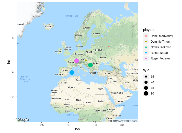
As we see, we can produce various output using dataframe objects.
A Basic Probability and Statistics with R
Wickham, Hadley. 2014a. Advanced R. CRC Press. http://adv-r.had.co.nz/.