An Introduction to Statistical Programming Methods with R
2020-10-20
Chapter 1 Introduction
This book is an early version of an ongoing project to equip students with the basic knowledge to master “statistical programming” with R.
The statistical software R has come into prominence due to its flexibility as an efficient language that builds a bridge between software development and data analysis. For example, one strength of R is the ease with which one can develop and quickly adapt to the different needs coming from the data management and analysis community while at the same time making use of other languages in order to deliver computationally efficient solutions. This book intends to present an approachable framework to statistical programming and software development using the wide variety of tools made available through R, from method-specific packages to version control programs. The general goals of the book are therefore the following:
- introduce tools and workflows for reproducible research (R/RStudio, Git/GitHub, etc.);
- introduce principles of tidy data and tools for data wrangling;
- exploit data structures to appropriately manage data, computer memory and computations;
- data manipulation through controls, instructions, and tailored functions;
- develop new software tools including functions, Shiny applications, and packages;
- manage the software development process including version control, documentation (with embedded code), and dissemination for other users.
The rest of this introductory chapter will present the R software by explaining why it is used for this book and describing the basic notations and tools that need to be known in order to better grasp its contents.

To highlight our goals, we will roughly follow the process that is represented in the diagram above. Indeed, in many cases, an input (e.g. data source) is provided, and then we process, explore, and/or manipulate the data with R. Once this is done, we then can communicate our findings through websites, reports, slides, etc. using some combination of RMarkdown, R and/or Shiny. This process is not always sequential since we can often have new ideas or observations at any stage this process therefore bringing us back to exploring the data again.
1.1 R and RStudio
The statistical computing language R has become commonplace for many applications in industry, government and academia. Having started as an open-source language to make different statistical and analytical tools available to researchers and the general public, it steadily developed into one of the major software languages which not only allows to develop up-to-date, sound and flexible analytical tools, but also to include these tools within a framework which is well-integrated with other important languages and features. The latter aspect is amplified thanks to the development of the RStudio interface which provides a pleasant and functional user-interface for R as well as an efficient Integrated Development Environment (IDE) in which different programming languages, web-applications and other important tools are readily available to the user. In order to illustrate the relationship between R and RStudio in statistical programming, one might think of a car analogy in which R would be the drivetrain and chassis while RStudio adds bluetooth, vocal commands, comfortable seats and air conditioning. R is doing most of the work, and the user can basically get where they want to go using R without RStudio, but RStudio is generally making you more comfortable while you use R (although you won’t get very far using RStudio without R).
1.1.1 Getting started with R
Since R is a free and open-source software, you may simply download it from the following link:
While R certainly can be used “as is” for many purposes, we strongly recommend using an IDE called RStudio. There are several versions of RStudio for different users (RStudio Desktop, Commercial, Server, etc.). The free RStudio Desktop version is sufficient for our purposes. RStudio can downloaded from the following link:
RStudio without having installed R on your computer.
1.1.2 Why R?
There are many reasons to use R. Two compelling reasons are that R is both free as in “free pizza”, and free as in “free speech”. Free–like “free pizza”–means that there is never a need to pay for any part of the R software, or contributed packages (i.e. add-on modules). Free–like “free speech”–means that there are very few restrictions on how R can be used or barriers to those who would like to contribute packages (i.e. add-on modules).
The fact that is a free and open-source software does not necessarily imply that it is a good software (although it is also that). The reason why this is an important feature consists in the fact that the results of any code or program developed in the R environment can easily be replicated therefore ensuring accessibility and transparency for the general user. More importantly however, this replicability of results is also accompanied by a wide variety of packages that are made available through the R environment in which users can find a diversity of codes, functions, and features that are designed to tackle a large amount of programming and analytical tasks. Moreover, new packages are relatively simple to create and are extremely useful for code-sharing purposes since they enclose the codes, functions, and external dependencies that allow anyone to easily and efficiently install these features. Additionally, these accessibility and code-sharing features have established R as a platform for development and dissemination of cutting-edge tools directly from the developer to the end-user.
1.1.3 About RStudio
RStudio is a customizable IDE for the R enviornment where the user can have easy access to plots, data, help, files, objects and many other features that are useful to work efficiently with R. For the most part, RStudio provides nearly everything the R user will need in a self-contained, and well-organized environment. Moreover, it is possible to create “projects” in which it is possible to create a dedicated environment space for sets of specific functions and files aimed to deal with various tasks.
Below is short video demonstrating a basic introduction of RStudio and some of its elements.
In addition, RStudio provides embedded functionality to utilize collaborative version-control software including GitHub & Subversion as well as a set of powerful tools to save and communicate results (whether they be simulations, data analysis, or presenting and making available a new package to other users). Some examples of these tools are Rmarkdown which can be used respectively to integrate written narrative with embedded R code and other content, as well as and Shiny Web Apps which can provide an interactive user-friendly interface that permits a user to actively engage with a wide variety of tools built in R without the need to encounter raw R code. GitHub and Rmarkdown will be the object of a more in-depth description in the first chapters of this book in order to provide the reader with the version-control and annotation tools that can be useful for the following chapters of this book.
1.1.4 Conventions
Throughout this book, R code will be typeset using a monospace font which is syntax highlighted. For example:
Similarly, R output lines (that usally appear in your Console) will begin with ## and will not be syntax highlighted. The output of the above example is the following:
## [1] 1Aside from R code and output, this book will also insert boxes in order to draw the reader’s attention to important, curious, or otherwise informative details. An example of these boxes was seen at the beginning of this introduction where an important aspect was pointed out to the reader regarding the “under construction” nature of this book. Therefore the following boxes and symbols can be used to represent information of different nature:
1.1.5 Getting help
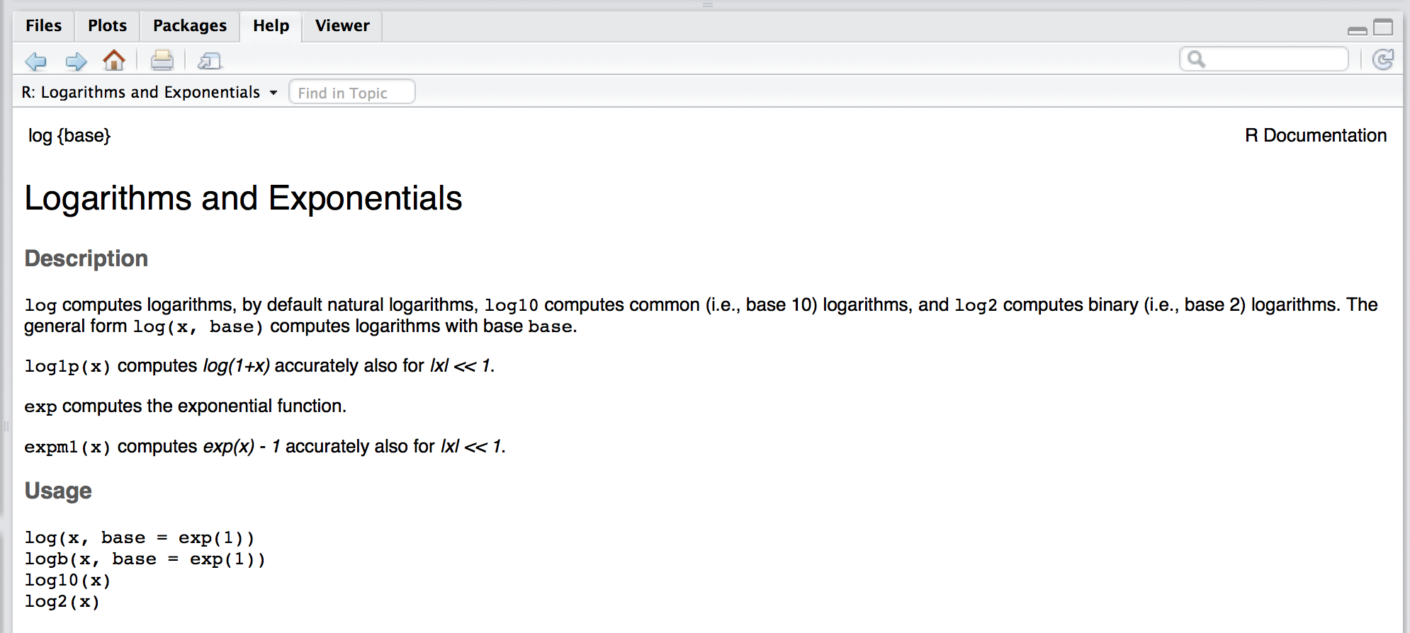
In the previous section we presented some examples on how R can be used as a calculator and we have already seen several functions such as sqrt() or log(). To obtain documentation about a function in R, simply put a question mark in front of the function name (or just type help() around the function name), or use the search bar on the “Help” tab in your RStudio window, and its documentation will be displayed. For example, if you are interested in learning about the function log() you could simply type:
which will display something similar to:
The R documentation is written by the author of the package. For mainstream packages in widespread use, the documentation is almost always quite good, but in some cases it can be quite technical, difficult to interpret, and possibly incomplete. In these cases, the best solution to understand a function is to search for help on any search engine. Often a simple search like “side by side boxplots in R” or “side by side boxplots in ggplot2” will produce many useful results. The search results often include user forums such as “CrossValidated” or “StackExchange” in which the questions you have about a function have probably already been asked and answered by many other users.
1.1.6 Installing packages
R comes with a number of built-in functions but one of its main strengths is that there is a large number of packages on an ever-increasing range of subjects available for you to install. These packages provide additional functions, features and data to the R environement. If you want to do something in R that is not available by default, there is a good chance that there are packages that will respond to your needs. In this case, an appropriate way to find a package in R is to use the search option in the CRAN repository which is the official network of file-transfer protocols and web-servers that store updated versions of code and documentation for R (see CRAN website). Another general approach to find a package in R is simply to use a search engine in which to type the keywords of the tools you are looking for followed by “R package”.
R packages can be installed in various ways but the most widely used approach is through the install.packages() function. Another way is to use the “Tools -> Install Packages…” path from the dropdown menus in RStudio or clicking on the “install” button in the “Packages” pane in the RStudio environment. The install.packages() function is very straight-forward and transcends any platform for the R environment. It is noteworthy that this approach assumes that the desired package(s) are available within the CRAN repository. This is very often the case, but there is a growing number of packages that are under-development or completed and are made available through other repositories. In the latter setting, Chapter 02 will show other ways of installing packages from a commonly used repository called “GitHub”.
Sticking momentarily to the packages available in the CRAN repository, the use of the install.packages() is quite simple. For example, if you want to install the package devtools you can simply write:
Once a package is installed it is not directly usable within your R session. To do so you will have to “load” the package into your current R session which is generally done through the function library(). For example, after having installed the devtools package, in order to use it within your session you would write:
Once this is done, all the functions and documentation of this package are available and can be used within your current session. However, once you close your R session, all loaded packages will be closed and you will have to load them again if you want to use them in a new R session.
One of the main packages that is required for this class would be our introDS package, that contains all the necessary packages and functions that will be utilized in this book. Run the following code to install the package directly from GitHub.
1.1.7 Additional References
There are many more elements in RStudio, and we encourage you to use the RStudio Cheatsheet as a reference.
1.2 Basic Probability and Statistics with R
The R environment provides an up-to-date and efficient programming language to develop different tools and applications. Nevertheless, its main functionality lies in the core statistical framework and tools that consistute the basis of this language. Indeed, this book aims at introducing and describing the methods and approaches of statistical programming which therefore require a basic knowledge of Probability and Statistics in order to grasp the logic and usefulness of the features presented in this book.
For this reason, we will briefly take the reader through some of the basic functions that are available within R to obtain probabilities based on parametric distributions, compute summary statistics and understand basic data structures. The latter is just an introduction and a more in-depth description of different data structures will be given in a future chapter.
1.2.1 Simple calculations
Since the R environment can serve as an advanced calculator, it is worth noting this also allows for simple calculations. In the table below we show a few examples of such calculations where the first column gives a mathematical expression (calculation), the second gives the equivalent of this expression in R and finally in the third column we can find the result that is output from R.
| Math. | R | Result |
|---|---|---|
| 2+2 | 2+2 |
4 |
| \(\frac{4}{2}\) | 4/2 |
2 |
| \(3 \cdot 2^{-0.8}\) | 3*2^(-0.8) |
1.723048 |
| \(\sqrt{2}\) | sqrt(2) |
1.414214 |
| \(\pi\) | pi |
3.141593 |
| \(\ln(2)\) | log(2) |
0.6931472 |
| \(\log_{3}(9)\) | log(9, base = 3) |
2 |
| \(e^{1.1}\) | exp(1.1) |
3.004166 |
| \(\cos(\sqrt{0.9})\) | cos(sqrt(0.9)) |
0.5827536 |
1.2.2 Probability Distributions
Probability distributions can be uniquely characterized by different functions such as, for example, their density or distribution functions. Based on these it is possible to compute theoretical quantiles and also randomly sample observations from them. Replacing the R syntax for a given probability distribution with the general syntax name, all these functions and calculations are made available in R through the built-in functions:
dnamecalculates the value of the density function (pdf);pnamecalculates the value of the distribution function (cdf);qnamecalculates the value of the theoretical quantile;rnamegenerates a random sample from a particular distribution.
Note that, when using these functions in practice, name is replaced with the syntax used in R to denote a specific probability distribution. For example, if we wish to deal with a Uniform probability distribution, then the syntax name is replaced by unif and, furthering the example, to randomly generate observations from a uniform distribution the function to use will be therefore runif. R allows to make use of these functions for a wide variety of probability distributions that include, but are not limited to: Gaussian (or Normal), Binomial, Chi-square, Exponential, F-distribution, Geometric, Poisson, Student-t and Uniform. In order to get an idea of how these functions can be used, below is an example of a problem that can be solved using them.
1.2.2.1 Example: Normal Test Scores of College Entrance Exam
Assume that the test scores of a college entrance exam follows a Normal distribution. Furthermore, suppose that the mean test score is 70 and that the standard deviation is 15. How would we find the percentage of students scoring 90 or more in this exam?
In this case, we consider a random variable \(X\) that is normally distributed as follows: \(X \sim N(\mu=70, \sigma^2=225)\) where \(\mu\) and \(\sigma^2\) represent the mean and variance of the distribution respectively. Since we are looking for the probability of students scoring higher than 90, we are interested in finding \(\mathbb{P}(X > x=90)\) and therefore we look at the upper tail of the Normal distribution. To find this probability we need the distribution function (pname) for which we therefore replace name with the R syntax for the Normal distribution: norm. The distribution function in R has various parameters to be specified in order to compute a probability which, at least for the Normal distribution, can be found by typing ?pnorm in the Console and are:
q: the quantile we are interested in (e.g. 90);mean: the mean of the distribution (e.g. 70);sd: the standard deviation of the distribution (e.g. 15);lower.tail: a boolean determining whether to compute the probability of being smaller than the given quantile (i.e. \(\mathbb{P}(X \leq x)\)) which requires the default argumentTRUEor larger (i.e. \(\mathbb{P}(X > x)\)) which requires to specify the argumentFALSE.
Knowing these arguments, it is now possible to compute the probability we are interested in as follows:
## [1] 0.09121122As we can see from the output, there is roughly a 9% probability of students scoring 90 or more on the exam.
1.2.3 Summary Statistics
While the previous functions deal with theoretical distributions, it is also necessary to deal with real data from which we would like to extract information. Supposing–as is often the case in applied statistics–we don’t know from which distribution it is generated, we would be interested in understanding the behavior of the data in order to eventually identify a distribution and estimate its parameters.
The use of certain functions varies according to the nature of the inputs since these can be, for example, numerical or factors.
1.2.3.1 Numerical Input
A first step in analysing numerical inputs is given by computing summary statistics of the data which, in this section, we can generally denote as x (we will discuss the structure of this data more in detail in the following chapters). For central tendency or spread statistics of a numerical input, we can use the following R built-in functions:
meancalculates the mean of an inputx;mediancalculates the median of an inputx;varcalculates the variance of an inputx;sdcalculates the standard deviation of an inputx;IQRcalculates the interquartile range of an inputx;mincalculates the minimum value of an inputx;maxcalculates the maximum value of an inputx;rangereturns a vector containing the minimum and maximum of all given arguments;summaryreturns a vector containing a mixture of the above functions (i.e. mean, median, first and third quartile, minimum, maximum).
1.2.3.2 Factor Input
If the data of interest is a factor with different categories or levels, then different summaries are more appropriate. For example, for a factor input we can extract counts and percentages to summarize the variable by using table. Using functions and data structures that will be described in the following chapters, below we create an example dataset with 90 observations of three different colors: 20 being Yellow, 10 being Green and 50 being Blue. We then apply the table function to it:
##
##   Blue  Green Yellow
##     50     10     20
By doing so we obtain a frequency (count) table of the colors.
1.2.3.3 Dataset Inputs
In many cases, when dealing with data we are actually dealing with datasets (see Chapter 03) where variables of different nature are aligned together (usually in columns). For datasets there is another convenient way to get simple summary statistics which consists in applying the function summary to the dataset itself (instead of simply a numerical input as seen earlier).
As an example, let us explore the Iris flower dataset contained in the R built-in datasets package. The data set consists of 50 samples from each of three species of Iris (Setosa, Virginica and Versicolor). Four features were measured from each sample consisting in the length and the width (in centimeters) of the both sepals and petals. This dataset is widely used as an example since it was used by Fisher to develop a linear discriminant model based on which he intended to distinguish the three species from each other using combinations of these four features.
Using this dataset, let us use the summary function on it to output the minimum, first quartile and thrid quartile, median, mean and maximum statistics (for the numerical variables in the dataset) and frequency counts (for factor inputs).
##   Sepal.Length    Sepal.Width     Petal.Length    Petal.Width
##  Min.   :4.300   Min.   :2.000   Min.   :1.000   Min.   :0.100
##  1st Qu.:5.100   1st Qu.:2.800   1st Qu.:1.600   1st Qu.:0.300
##  Median :5.800   Median :3.000   Median :4.350   Median :1.300
##  Mean   :5.843   Mean   :3.057   Mean   :3.758   Mean   :1.199
##  3rd Qu.:6.400   3rd Qu.:3.300   3rd Qu.:5.100   3rd Qu.:1.800
##  Max.   :7.900   Max.   :4.400   Max.   :6.900   Max.   :2.500
##        Species
##  setosa    :50
##  versicolor:50
##  virginica :50
##
##
##
1.3 Main References
This is not the first (or the last) book that has been written explaining and describing statistical programming in R. Indeed, this can be seen as a book that brings together and reorganizes information and material from other sources structuring and tailoring it to a course in basic statistical programming. The main references (which are far from being an exhaustive review of literature) that can be used to have a more in-depth view of different aspects treated in this book are:
1.4 License
You can redistribute it and/or modify this book under the terms of the Creative Commons Attribution-NonCommercial-ShareAlike 4.0 International License (CC BY-NC-SA) 4.0 License.