Allan Variance Linear Regression Estimation Examples

2020-01-21

library(avar)

Simulated Data

To understand the features of the avar package, we first illustrate with a simulated data of sample size \(n = 10^5\) coming from a White Noise (WN) plus Random Walk (RW) model. The corresponding (maximum-overlap) Allan Variance representation is given in the following figure:

set.seed(2710)

# Simulate data
n = 1e5
data = rnorm(n, 0, 0.01) +  cumsum(rnorm(n, 0, 3.162278e-05))

# Compute the Maximum-Overlap Allan Variance
allan_variance = avar(data, type = "mo")

# Log-Log representation of the Allan Variance
plot(allan_variance)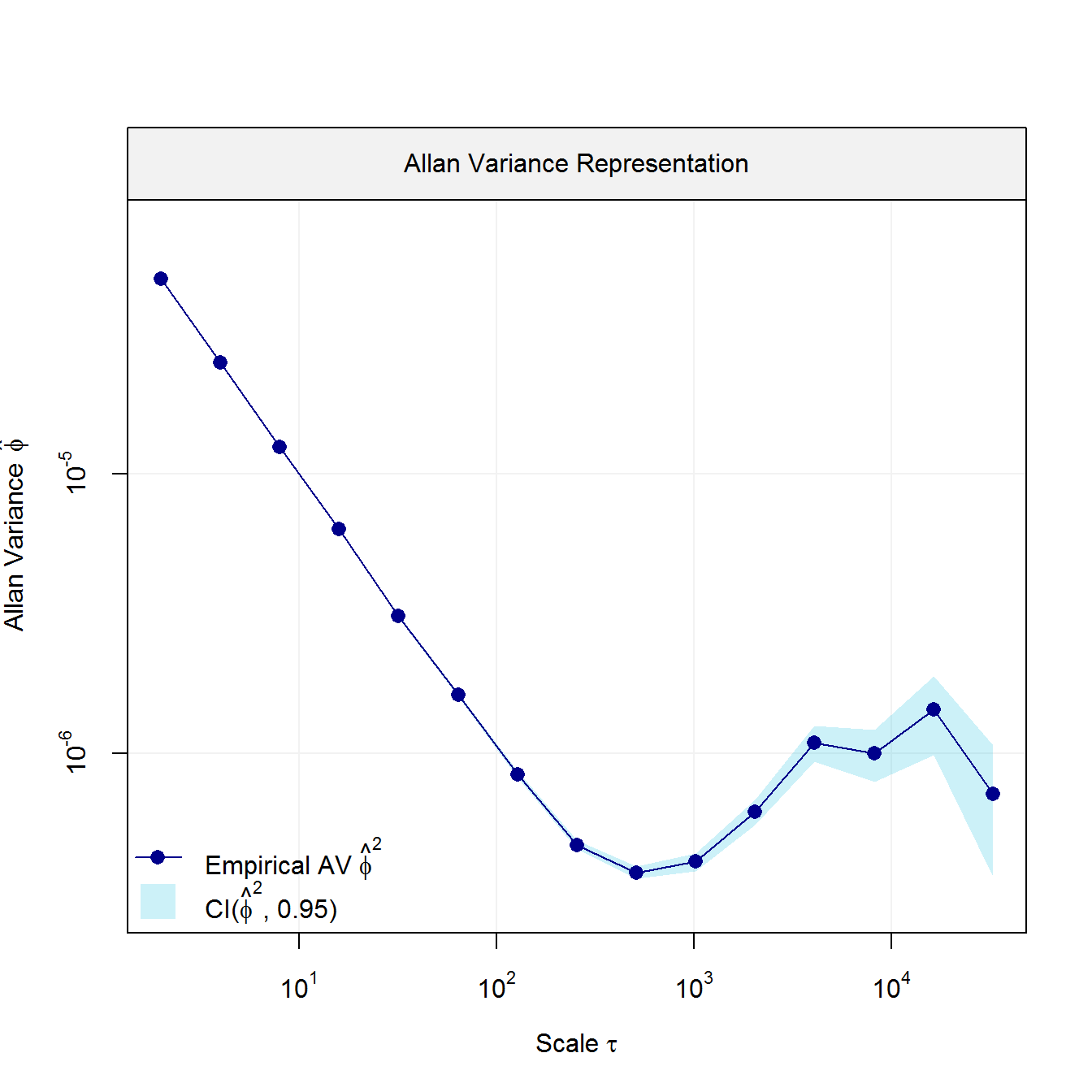

Allan Variance Representation.

Based on this graph, it is possible to detect the models underlying the simulated data. Indeed, we can see that our model should include a WN process when considering the first 7 scales and a RW process when considering the last 3 scales. Therefore, using these scales we can make use of the traditional “Allan Variance slope method” to estimate the parameters of these two processes.

# Specify the scale at which we want to fit the WN and RW processes
wn = 1:7
rw = 13:15

# Compute the Allan Variance Linear Regression Estimator (AVLR)
fit = avlr(allan_variance, wn = wn, rw = rw)
fit
#> 
#>  Estimates: 
#>           Value
#> WN 1.007431e-02
#> RW 1.358511e-05

Now that we have computed the parameters of interest, we can visually check if the chosen latent model fits the data at hand well. To do so we can simply use the plot function and, if we would like to observe how the individual processes contribute to the overall fit, we can set the parameter decomp = TRUE.

plot(fit)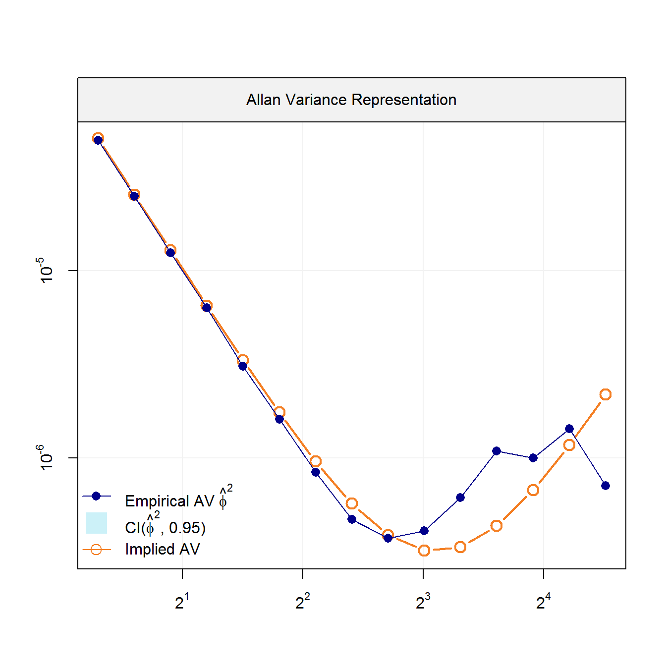

Empirical AV with AV implied by the latent model

plot(fit, decomp = TRUE)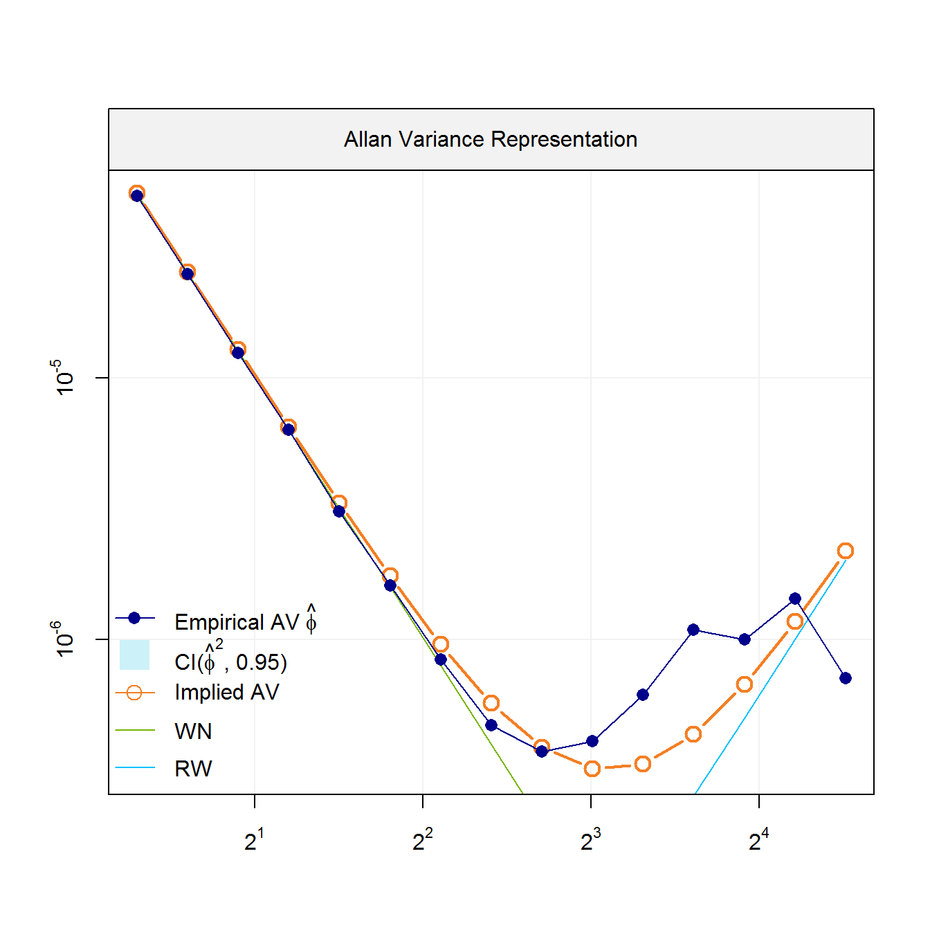

Empirical AV with AV implied by the latent model

As we can see, the model fits the data well. Therefore, we are going to compute the confidence intervals for these parameters by specifiying the option ci = TRUE. These confidence intervals are computed via parametric bootstrap for which the number of replications can be defined through the parameter B.

# AVLR estimator with 95% confidence intervals
fit_ci = avlr(allan_variance, wn = 1:7, rw = 13:15, ci = TRUE, B = 100)
fit_ci$ci

#> $mu
#> [1] 0.0100782190 0.0000121613
#> 
#> $ci
#>              [,1]         [,2]
#> [1,] 1.005670e-02 1.008411e-02
#> [2,] 1.392184e-05 1.609601e-05
#> 
#> $sd
#> [1] 5.526008e-05 4.383085e-06

Real IMU Data

We can further illustrate the features of the avar package using the Allan variance computed based on real IMU data. Specifically, we consider the Allan variance of IMU data collected from a navchip sensor, i.e. navchip_av, whose sample size is about \(n = 3 \cdot 10^6\). The Allan variance representation corresponding to this dataset is given in the following figure:

data("navchip_av")
plot(navchip_av)

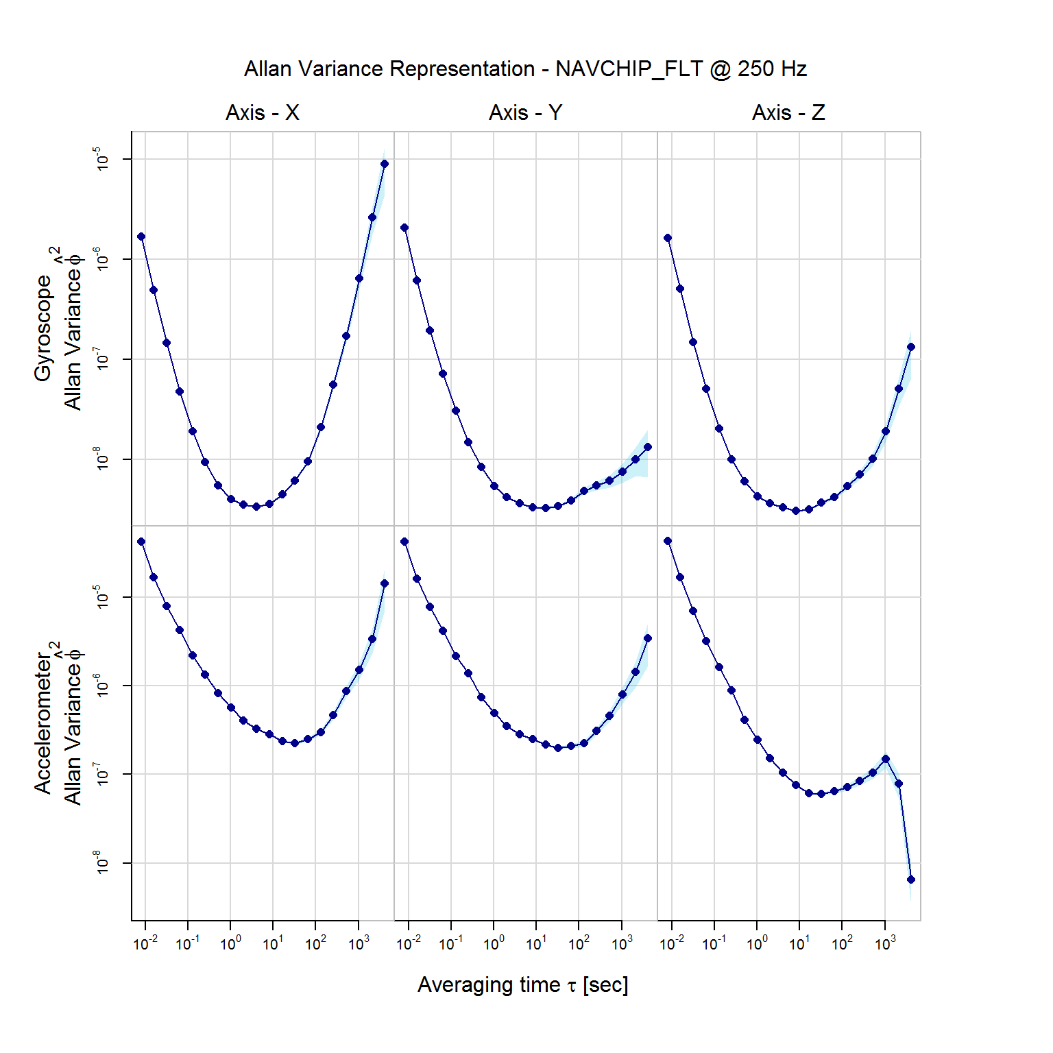
Allan Variance Representation.

Based on the graph, we can see that for the gyroscope components, the underlying model should include a Quantization Noise (QN) for the first 4 scales, a WN for the 6th to 8th scales, and a RW for the 10th to 13th scales. Similarly for the accelerometer components, the underlying model should include a WN for the first 6 scales and a RW for the 14th to 16th scales. Therefore, we can estimate the underlying model with the following:

fit2 = avlr(navchip_av, qn_gyro = 1:4, wn_gyro = 6:8, rw_gyro = 10:13,
           wn_acc = 1:6, rw_acc = 14:16)
fit2
#> 
#>  Estimates for gyroscopes: 
#>           Value
#> WN 5.945877e-05
#> QN 7.208553e-06
#> RW 3.062325e-05
#> 
#>  Estimates for accelerometers: 
#>           Value
#> WN 5.233402e-04
#> RW 6.422082e-05

And we can visualize to check if the estimated underlying model fits the data well simply with the plot function.

plot(fit2)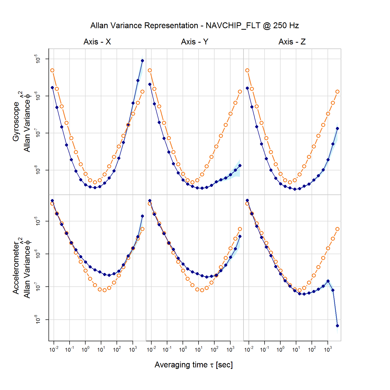

Empirical AV with AV implied by the latent model