Chapter 4 The Family of Autoregressive Moving Average Models
“Essentially, all models are wrong, but some are useful”, George Box
In this chapter we introduce a class of time series models that is considerably flexible and among the most commonly used to describe stationary time series. This class is represented by the Seasonal AutoRegressive Integrated Moving Average (SARIMA) models which, among others, combine and include the autoregressive and moving average models seen in the previous chapter. To introduce this class of models, we start by describing a sub-class called AutoRegressive Moving Average (ARMA) models which represent the backbone on which the SARIMA class is built. The importance of ARMA models resides in their flexibility as well as their capacity of describing (or closely approximating) almost all the features of a stationary time series. The autoregressive parts of these models describe how consecutive observations in time influence each other while the moving average parts capture some possible unobserved shocks thereby allowing to model different phenomena which can be observed in various fields going from biology to finance.
With this premise, the first part of this chapter introduces and explains the class of ARMA models in the following manner. First of all we will discuss the class of linear processes, which ARMA models belong to, and we will then proceed to a detailed description of autoregressive models in which we review their definition, explain their properties, introduce the main estimation methods for their parameters and highlight the diagnostic tools which can help understand if the estimated models appear to be appropriate or sufficient to well describe the observed time series. Once this is done, we will then use most of the results given for the autoregressive models to further describe and discuss moving average models, for which we underline the property of invertibility, and finally the ARMA models. Indeed, the properties and estimation methods for the latter class are directly inherited from the discussions on the autoregressive and moving average models.
The second part of this chapter introduces the general class of SARIMA models, passing through the class of ARIMA models. These models allow to apply the ARMA modeling framework also to time series that have particular non-stationary components to them such as, for example, linear and/or seasonal trends. Extending ARMA modeling to these cases allows SARIMA models to be an extremely flexible class of models that can be used to describe a wide range of phenomena.
4.1 Linear Processes
In order to discuss the classes of models mentioned above, we first present the class of linear processes which underlie many of the most common time series models.
Definition 4.1 (Linear Process) A time series, \((X_t)\), is defined to be a linear process if it can be expressed as a linear combination of white noise as follows:
\[{X_t} = \mu + \sum\limits_{j = - \infty }^\infty {{\psi _j}{W_{t - j}}} \]
where \(W_t \sim \mathcal{N}(0, \sigma^2)\) and \(\sum\limits_{j = - \infty }^\infty {\left| {{\psi _j}} \right|} < \infty\).
Note, the latter assumption is required to ensure that the series has a limit. Furthermore, the set of coefficients \[{( {\psi _j}) _{j = - \infty , \cdots ,\infty }}\] can be viewed as a linear filter. These coefficients do not have to be all equal nor symmetric as later examples will show. Generally, the properties of a linear process related to mean and variance are given by:
\[\begin{aligned} \mu_{X} &= \mu \\ \gamma_{X}(h) &= \sigma _W^2\sum\limits_{j = - \infty }^\infty {{\psi _j}{\psi _{h + j}}} \end{aligned}\]
The latter is derived from
\[\begin{aligned} \gamma \left( h \right) &= Cov\left( {{x_t},{x_{t + h}}} \right) \\ &= Cov\left( {\mu + \sum\limits_{j = - \infty }^\infty {{\psi _j}{w_{t - j}}} ,\mu + \sum\limits_{j = - \infty }^\infty {{\psi _j}{w_{t + h - j}}} } \right) \\ &= Cov\left( {\sum\limits_{j = - \infty }^\infty {{\psi _j}{w_{t - j}}} ,\sum\limits_{j = - \infty }^\infty {{\psi _j}{w_{t + h - j}}} } \right) \\ &= \sum\limits_{j = - \infty }^\infty {{\psi _j}{\psi _{j + h}}Cov\left( {{w_{t - j}},{w_{t - j}}} \right)} \\ &= \sigma _w^2\sum\limits_{j = - \infty }^\infty {{\psi _j}{\psi _{j + h}}} \\ \end{aligned} \]
Within the above derivation, the key is to realize that \(Cov\left( {{w_{t - j}},{w_{t + h - j}}} \right) = 0\) if \(t - j \ne t + h - j\).
Lastly, another convenient way to formalize the definition of a linear process is through the use of the backshift operator (or lag operator) which is itself defined as follows:
\[B\,X_t = X_{t-1}.\]
The properties of the backshift operator allow us to create composite functions of the type
\[B^2 \, X_t = B (B \, X_t) = B \, X_{t-1} = X_{t-2}\] which allows to generalize as follows
\[B^k \, X_t = X_{t-k}.\] Moreover, we can apply the inverse operator to it (i.e. \(B^{-1} \, B = 1\)) thereby allowing us to have, for example:
\[X_t = B^{-1} \, B X_t = B^{-1} X_{t-1}\]
Having defined the backshift operator, we can now provide an alternative definition of a linear process as follows:
\[{X_t} = \mu + \psi \left( B \right){W_t}\]
where \(\psi ( B )\) is a polynomial function in \(B\) whose coefficients are given by the linear filters \((\psi_j)\) (we’ll describe these polynomials further on).
Example 4.2 (Linear Process of White Noise) The white noise process \((X_t)\), defined in 2.4.1, can be expressed as a linear process as follows:
\[\psi _j = \begin{cases} 1 , &\mbox{ if } j = 0\\ 0 , &\mbox{ if } |j| \ge 1 \end{cases}.\]
and \(\mu = 0\).
Therefore, \(X_t = W_t\), where \(W_t \sim WN(0, \sigma^2_W)\)
Example 4.3 (Linear Process of Moving Average Order 1) Similarly, consider \((X_t)\) to be a MA(1) process, given by 2.4.4. The process can be expressed linearly through the following filters:
\[\psi _j = \begin{cases} 1, &\mbox{ if } j = 0\\ \theta , &\mbox{ if } j = 1 \\ 0, &\mbox{ if } j \ge 2 \end{cases}.\]
and \(\mu = 0\).
Thus, we have: \(X_t = W_t + \theta W_{t-1}\)
Example 4.4 (Linear Process and Symmetric Moving Average) Consider a symmetric moving average given by:
\[{X_t} = \frac{1}{{2q + 1}}\sum\limits_{j = - q}^q {{W_{t + j}}} \]
Thus, \((X_t)\) is defined for \(q + 1 \le t \le n-q\). The above process would be a linear process since:
\[\psi _j = \begin{cases} \frac{1}{{2q + 1}} , &\mbox{ if } -q \le j \le q\\ 0 , &\mbox{ if } |j| > q \end{cases}.\]
and \(\mu = 0\).
In practice, if \(q = 1\), we would have:
\[{X_t} = \frac{1}{3}\left( {{W_{t - 1}} + {W_t} + {W_{t + 1}}} \right)\]
Example 4.5 (Autoregressive Process of Order 1) If \(\left\{X_t\right\}\) follows an AR(1) model defined in 2.4.3, the linear filters are a function of the time lag:
\[\psi _j = \begin{cases} \phi^j , &\mbox{ if } j \ge 0\\ 0 , &\mbox{ if } j < 0 \end{cases}.\]
and \(\mu = 0\). We would require the condition that \(\left| \phi \right| < 1\) in order to respect the condition on the filters (i.e. \(\sum\limits_{j = - \infty }^\infty {\left| {{\psi _j}} \right|} < \infty\)).4.2 Autoregressive Models - AR(p)
The class of autoregressive models is based on the idea that previous values in the time series are needed to explain current values in the series. For this class of models, we assume that the \(p\) previous observations are needed for this purpose and we therefore denote this class as AR(\(p\)). In the previous chapter, the model we introduced was an AR(1) in which only the immediately previous observation is needed to explain the following one and therefore represents a particular model which is part of the more general class of AR(\(p\)) models.
As earlier in this book, we will assume that the expectation of the process \(({X_t})\), as well as that of the following ones in this chapter, is zero. The reason for this simplification is that if \(\mathbb{E} [ X_t ] = \mu\), we can define an AR process around \(\mu\) as follows:
\[X_t - \mu = \sum_{i = 1}^p \phi_i \left(X_{t-i} - \mu \right) + W_t,\]
which is equivalent to
\[X_t = \mu^{\star} + \sum_{i = 1}^p \phi_i X_{t-i} + W_t,\]
where \(\mu^{\star} = \mu (1 - \sum_{i = 1}^p \phi_i)\). Therefore, to simplify the notation we will generally consider only zero mean processes, since adding means (as well as other deterministic trends) is easy.
A useful way of representing AR(\(p\)) processes is through the backshift operator introduced in the previous section and is as follows
\[\begin{aligned} {X_t} &= {\phi_1}{X_{t - 1}} + ... + {\phi_p}{X_{t - p}} + {W_t} \\ &= {\phi_1}B{X_t} + ... + {\phi_p}B^p{X_t} + {W_t} \\ &= ({\phi_1}B + ... + {\phi_p}B^p){X_t} + {W_t} \\ \end{aligned},\]
which finally yields
\[(1 - {\phi _1}B - ... - {\phi_p}B^p){X_t} = {W_t},\]
which, in abbreviated form, can be expressed as
\[\phi(B){X_t} = W_t.\]
We will see that \(\phi(B)\) is important to establish the stationarity of these processes and is called the autoregressive operator. Moreover, this quantity is closely related to another important property of AR(p) processes called causality. Before formally defining this new property we consider the following example which provides an intuitive illustration of its importance.
Example: Consider a classical AR(1) model with \(|\phi| > 1\). Such a model could be expressed as
\[X_t = \phi^{-1} X_{t+1} - \phi^{-1} W_t = \phi^{-k} X_{t+k} - \sum_{i = 1}^{k-1} \phi^{-i} W_{t+i}.\]
Since \(|\phi| > 1\), we obtain
\[X_t = - \sum_{j = 1}^{\infty} \phi^{-j} W_{t+j},\]
which is a linear process and therefore is stationary. Unfortunately, such a model is useless because we need the future to predict the future. These processes are called non-causal.
4.2.1 Properties of AR(p) models
In this section we will describe the main property of the AR(p) model which has already been mentioned in the previous paragraphs and therefore let us now introduce the property of causality in a more formal manner.
Definition: An AR(p) model is causal if the time series \((X_t)_{-\infty}^{\infty}\) can be written as a one-sided linear process: \[\begin{equation} X_t = \sum_{j = 0}^{\infty} \psi_j W_{t-j} = \frac{1}{\phi(B)} W_t = \psi(B) W_t, \tag{4.1} \end{equation}\]where \(\phi(B) = \sum_{j = 0}^{\infty} \phi_j B^j\), and \(\sum_{j=0}^{\infty}|\phi_j| < \infty\) and setting \(\phi_0 = 1\).
As discussed earlier this condition implies that only the past values of the time series can explain the future values of it and not viceversa. Moreover, given the expression of the linear filters given by \[\frac{1}{\phi(B)}\] it is obvious that a solution exists only when \(\phi(B) = \sum_{j = 0}^{\infty} \phi_j B^j \neq 0\) (thereby implying causality). A condition for this to be respected is for the roots of \(\phi(B) = 0\) to lie outside the unit circle.
Example 4.6 (Transform an AR(2) into a Linear Process) Consider an AR(2) process \[X_t = 1.3 X_{t-1} - 0.4 X_{t-2} + W_t,\] which we would like to transform into a linear process. This can be done using the following approach:
Step 1: The autoregressive operator of this model can be expressed as \[ \phi(B) = 1-1.3B+0.4B^2 = (1-0.5B)(1-0.8B), \] and has roots 2 and 1.25, both \(>1\). Thus, we should be able to convert it into a linear process.
Step 2: We know that if an AR(p) process has all its roots outside the unit circle, then we can write \(X_t = \frac{1}{\phi(B)} W_t\). By applying the partial fractions trick, we can inverse the autoregressive operator \(\phi(B)\) as follows: \[ \begin{aligned} \phi^{-1}(B) &= \frac{1}{(1-0.5B)(1-0.8B)} = \frac{c_1}{(1-0.5B)} + \frac{c_2}{(1-0.8B)} \\ &= \frac{c_2(1-0.5B) + c_1(1-0.8B)}{(1-0.5B)(1-0.8B)} = \frac{(c_1 + c_2)-(0.8c_1+0.5c_2)B}{(1-0.5B)(1-0.8B)}. \end{aligned} \]
To solve for \(c_1\) and \(c_2\): \[ \begin{cases} c_1 + c_2 &=1\\ 0.8c_1+0.5c_2 &=0 \end{cases} \to \begin{cases} c_1 &= -5/3\\ c_2 &= 8/3. \end{cases} \]
So we obtain \[ \phi^{-1}(B) = \frac{-5}{3(1-0.5B)} + \frac{8}{3(1-0.8B)}. \]
- Step 3: Using the Geometric series, i.e. \(a\sum_{j=0}^{\infty} r^j = \frac{a}{1-r}\) if \(|r| <1\), we have \[ \begin{cases} \frac{-5}{3(1-0.5B)} = -\frac{5}{3} \sum_{j=0}^\infty 0.5^j B^j, &\mbox{ if } |B| < 2 \\ \frac{8}{3(1-0.8B)} = \frac{8}{3} \sum_{j=0}^\infty 0.8^j B^j, &\mbox{ if } |B| < 1.25. \end{cases} \]
So we can express \(\phi^{-1}(B)\) as \[ \phi^{-1}(B) = \sum_{j=0}^\infty \Big[ -\frac{5}{3} (0.5)^j + \frac{8}{3} (0.8)^j \Big] B^j, \;\;\; \text{if } |B|<1.25. \]
- Step 4: Finally, we obtain \[ \begin{aligned} X_t &= \phi(B)^{-1} W_t = \sum_{j=0}^\infty \Big[ -\frac{5}{3} (0.5)^j + \frac{8}{3} (0.8)^j \Big] B^j W_t \\ &= \sum_{j=0}^\infty \Big[ -\frac{5}{3} (0.5)^j + \frac{8}{3} (0.8)^j \Big] W_{t-j}, \end{aligned} \] which verifies that the AR(2) is causal, and therefore is stationary.
Example 4.7 (Causal Conditions for an AR(2) Process) We already know that an AR(1) is causal with the simple condition \(|\phi_1|<1\). It seems natural to believe that an AR(2) should be causal (and therefore stationary) with the condition that \(|\phi_i| <1, \; i=1,2\). However, this is actually not the case as we illustrate below.
We can express an AR(2) process as \[ X_t = \phi_1 X_{t-1} + \phi_2 X_{t-2} + W_t = \phi_1 BX_t + \phi_2 B^2 X_t + W_t, \] thereby delivering the following autoregressive operator: \[ \phi(B) = 1-\phi_1 B - \phi_2 B^2 = \Big( 1-\frac{B}{\lambda_1} \Big) \Big( 1-\frac{B}{\lambda_2} \Big) \] where \(\lambda_1\) and \(\lambda_2\) are the roots of \(\phi(B)\) such that \[ \begin{aligned} \phi_1 &= \frac{1}{\lambda_1} + \frac{1}{\lambda_2}, \\ \phi_2 &= - \frac{1}{\lambda_1} \frac{1}{\lambda_2}. \end{aligned} \]
That is, \[\begin{aligned} \lambda_1 &= \frac{\phi_1 + \sqrt{\phi_1^2 + 4\phi_2}}{-2\phi_2}, \\ \lambda_2 &= \frac{\phi_1 - \sqrt{\phi_1^2 + 4\phi_2}}{-2\phi_2}. \end{aligned} \]
In order to ensure the causality of the model, we need the roots of \(\phi(B)\), i.e. \(\lambda_1\) and \(\lambda_2\), to lie outside the unit circle.
\[ \begin{cases} |\lambda_1| &> 1 \\ |\lambda_2| &> 1, \end{cases} \] if and only if \[ \begin{cases} \phi_1 + \phi_2 &< 1 \\ \phi_2 - \phi_1 &< 1 \\ |\phi_2| &<1. \end{cases} \]
We can show the if part of the statement as follows: \[ \begin{aligned} & \phi_1 + \phi_2 = \frac{1}{\lambda_1} + \frac{1}{\lambda_2} - \frac{1}{\lambda_1 \lambda_2} = \frac{1}{\lambda_1} \Big(1-\frac{1}{\lambda_2} \Big) + \frac{1}{\lambda_2} < 1 - \frac{1}{\lambda_2} + \frac{1}{\lambda_2} = 1 \;\; \text{since } 1-\frac{1}{\lambda_2} > 0, \\ & \phi_2 - \phi_1 = -\frac{1}{\lambda_1 \lambda_2} - \frac{1}{\lambda_1} - \frac{1}{\lambda_2} = -\frac{1}{\lambda_1} \Big( \frac{1}{\lambda_2} +1 \Big) - \frac{1}{\lambda_2} < \frac{1}{\lambda_2}+1-\frac{1}{\lambda_2} = 1 \;\; \text{since } \frac{1}{\lambda_2}+1 > 0, \\ & |\phi_2| = \frac{1}{|\lambda_1| |\lambda_2|} < 1. \end{aligned} \]
We can also show the only if part of the statement as follows:
Since \(\lambda_1 = \frac{\phi_1 + \sqrt{\phi_1^2 + 4\phi_2}}{-2\phi_2}\) and \(\phi_2 - 1 < \phi_1 < 1- \phi_2\), we have \[ \lambda_1^2 = \frac{(\phi_1 + \sqrt{\phi_1^2 + 4\phi_2})^2}{4\phi_2^2} < \frac{\Big( (1-\phi_2)+ \sqrt{(1-\phi_2)^2 + 4\phi_2} \Big)^2}{4\phi_2^2} = \frac{4}{4\phi_2^2} \leq 1. \]
Since \(\lambda_2 = \frac{\phi_1 - \sqrt{\phi_1^2 + 4\phi_2}}{-2\phi_2}\) and \(\phi_2 - 1 < \phi_1 < 1- \phi_2\), we have \[ \lambda_2^2 = \frac{(\phi_1 - \sqrt{\phi_1^2 + 4\phi_2})^2}{4\phi_2^2} < \frac{\Big( (\phi_2-1)+ \sqrt{(\phi_2-1)^2 + 4\phi_2} \Big)^2}{4\phi_2^2} = \frac{4\phi_2^2}{4\phi_2^2} = 1. \]
Finally, the causal region of an AR(2) is demonstrated as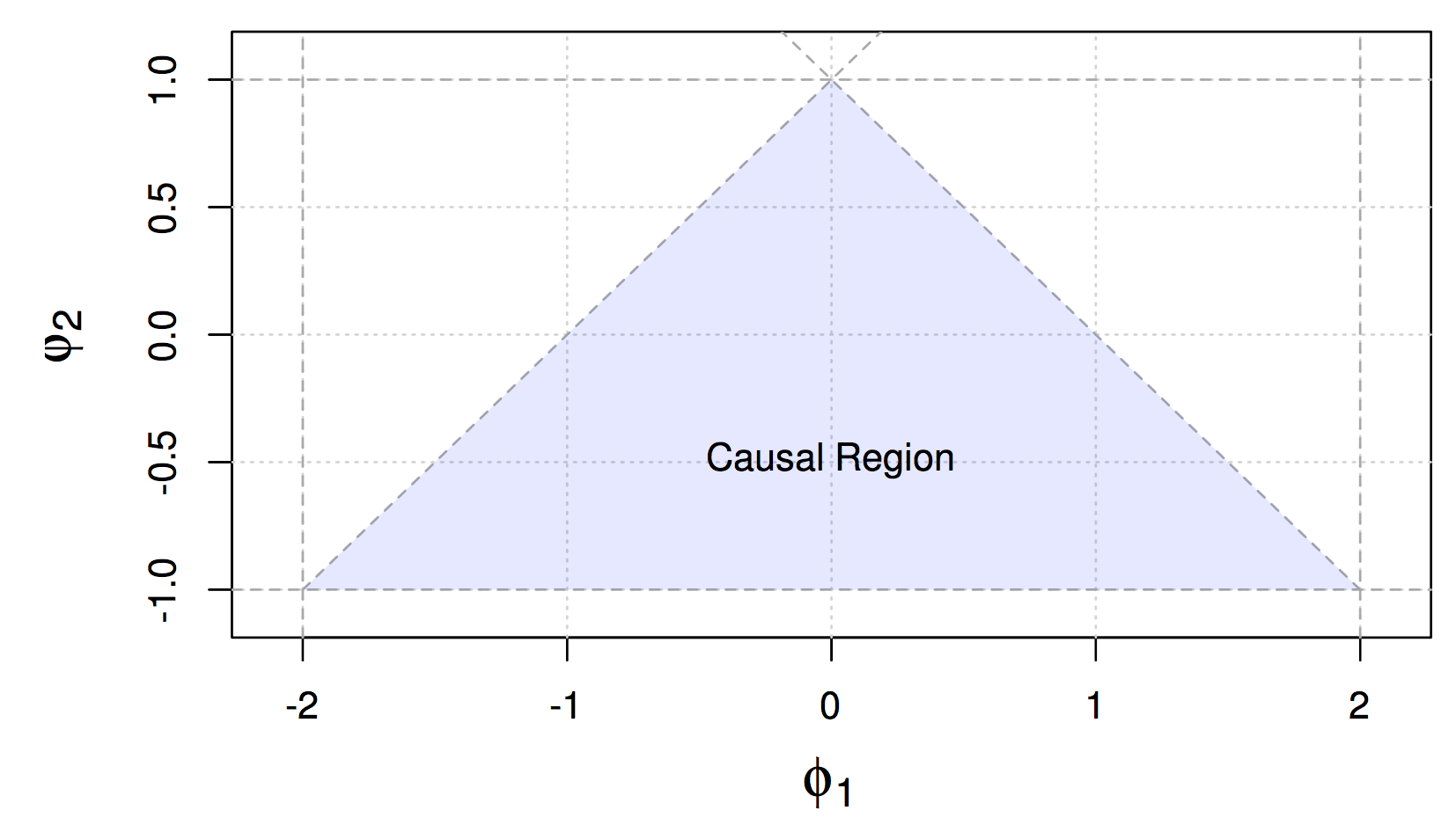
Figure 4.1: Causal Region for Parameters of an AR(2) Process
4.2.2 Estimation of AR(p) models
Given the above defined properties of AR(p) models, we will now discuss how these models can be estimated, more specifically how the \(p+1\) parameters can be obtained from an observed time series. Indeed, a reliable estimation of these models is necessary in order to intepret and describe different natural phenomena and/or forecast possible future values of the time series.
A first approach builds upon the earlier definition of AR(\(p\)) models being a linear process. Recall that \[\begin{equation} X_t = \sum_{j = 1}^{p} \phi_j X_{t-j} \end{equation}\] which delivers the following autocovariance function \[\begin{equation} \gamma(h) = \text{cov}(X_{t+h}, X_t) = \text{cov}\left(\sum_{j = 1}^{p} \phi_j X_{t+h-j}, X_t\right) = \sum_{j = 1}^{p} \phi_j \gamma(h-j), \mbox{ } h \geq 1. \end{equation}\] Rearranging the above expressions we obtain the following general equations \[\begin{equation} \gamma(h) - \sum_{j = 1}^{p} \phi_j \gamma(h-j) = 0, \mbox{ } h \geq 1 \end{equation}\] and, recalling that \(\gamma(h) = \gamma(-h)\), \[\begin{equation} \gamma(0) - \sum_{j = 1}^{p} \phi_j \gamma(j) = \sigma_w^2. \end{equation}\]We can now define the Yule-Walker equations.
Definition: The Yule-Walker equations are given by \[\begin{equation} \gamma(h) = \phi_1 \gamma(h-1) + ... + \phi_p \gamma(h-p), \mbox{ } h = 1,...,p \end{equation}\] and \[\begin{equation} \sigma_w^2 = \gamma(0) - \phi_1 \gamma(1) - ... - \phi_p \gamma(p). \end{equation}\] which in matrix notation can be defined as follows \[\begin{equation} \Gamma_p \mathbf{\phi} = \mathbf{\gamma}_p \,\, \text{and} \,\, \sigma_w^2 = \gamma(0) - \mathbf{\phi}'\mathbf{\gamma}_p \end{equation}\]where \(\Gamma_p\) is the \(p\times p\) matrix containing the autocovariances \(\gamma(k-j)\), where \(j,k = 1, ...,p\), while \(\mathbf{\phi} = (\phi_1,...,\phi_p)'\) and \(\mathbf{\gamma}_p = (\gamma(1),...,\gamma(p))'\) are \(p\times 1\) vectors.
Considering the Yule-Walker equations, it is possible to use a method of moments approach and simply replace the theoretical quantities given in the previous definition with their empirical (estimated) counterparts that we saw in the previous chapter. This gives us the following Yule-Walker estimators \[\begin{equation} \hat{\mathbf{\phi}} = \hat{\Gamma}_p^{-1}\hat{\mathbf{\gamma}}_p \,\, \text{and} \,\, \hat{\sigma}_w^2 = \hat{\gamma}(0) - \hat{\mathbf{\gamma}}_p'\hat{\Gamma}_p^{-1}\hat{\mathbf{\gamma}}_p . \end{equation}\]These estimators have the following asymptotic properties.
Consistency and Asymptotic Normality of Yule-Walker estimators: The Yule-Walker estimators for a causal AR(\(p\)) model have the following asymptotic properties:
\[\begin{equation*} \sqrt{T}(\hat{\mathbf{\phi}}- \mathbf{\phi}) \xrightarrow{\mathcal{D}} \mathcal{N}(\mathbf{0},\sigma_w^2\Gamma_p^{-1}) \,\, \text{and} \,\, \hat{\sigma}_w^2 \xrightarrow{\mathcal{P}} \sigma_w^2 . \end{equation*}\] Therefore the Yule-Walker estimators have an asymptotically normal distribution and the estimator of the innovation variance is consistent. Moreover, these estimators are also optimal for AR(\(p\)) models, meaning that they are also efficient. However, there is also another method which allows to achieve this efficiency (also for general ARMA models that will be tackled further on) and this is the Maximum Likelihood Estimation (MLE) method. Considering an AR(1) model as an example, and assuming without loss of generality that its expectation is zero, we have the following representation of the AR(1) model \[\begin{equation*} X_t = \phi X_{t-1} + W_t, \end{equation*}\] where \(|\phi|<1\) and \(W_t \overset{iid}{\sim} \mathcal{N}(0,\sigma_w^2)\). Supposing we have observations \((x_t)_{t=1,...,T}\) issued from this model, then the likelihood function for this setting is given by \[\begin{equation*} L(\phi,\sigma_w^2) = f(\phi,\sigma_w^2|x_1,...,x_T) \end{equation*}\] which, for an AR(1) model, can be rewritten as follows \[\begin{equation*} L(\phi,\sigma_w^2) = f(x_1)f(x_2|x_1)\cdot \cdot \cdot f(x_T|x_{T-1}). \end{equation*}\] If we define \(\Omega_t^p\) as the information contained in the previous \(p\) observations (before time \(t\)), the above expression can be generalized for an AR(p) model as follows \[\begin{equation*} L(\phi,\sigma_w^2) = f(x_1,...,x_p)f(x_{p+1}|\Omega_{p+1}^p)\cdot \cdot \cdot f(x_T|\Omega_{T}^p) \end{equation*}\] where \(f(x_1,...,x_p)\) is the joint probability distribution of the first \(p\) observations. Going back to the AR(1) setting, based on our assumption on \((W_t)\) we know that \(x_t|x_{t-1} \sim \mathcal{N}(\phi x_{t-1},\sigma_w^2)\) and therefore we have that \[\begin{equation*} f(x_t|x_{t-1}) = f_w(x_t - \phi x_{t-1}) \end{equation*}\] where \(f_w(\cdot)\) is the distribution of \(W_t\). This rearranges the likelihood function as follows \[\begin{equation*} L(\phi,\sigma_w^2) = f(x_1)\prod_{t=2}^T f_w(x_t - \phi x_{t-1}), \end{equation*}\] where \(f(x_1)\) can be found through the causal representation \[\begin{equation*} x_1 = \sum_{j=0}^{\infty} \phi^j w_{1-j}, \end{equation*}\] which implies that \(x_1\) follows a normal distribution with zero expectation and a variance given by \(\frac{\sigma_w^2}{(1-\phi^2)}\). Based on this, the likelihood function of an AR(1) finally becomes \[\begin{equation*} L(\phi,\sigma_w^2) = (2\pi \sigma_w^2)^{-\frac{T}{2}} (1 - \phi^2)^{\frac{1}{2}} \exp \left(-\frac{S(\phi)}{2 \sigma_w^2}\right), \end{equation*}\] with \(S(\phi) = (1-\phi^2) x_1^2 + \sum_{t=2}^T (x_t -\phi x_{t-1})^2\). Once the derivative of the logarithm of the likelihood is taken, the minimization of the negative of this function is usually done numerically. However, if we condition on the initial values, the AR(p) models are linear and, for example, we can then define the conditional likelihood of an AR(1) as \[\begin{equation*} L(\phi,\sigma_w^2|x_1) = (2\pi \sigma_w^2)^{-\frac{T-1}{2}} \exp \left(-\frac{S_c(\phi)}{2 \sigma_w^2}\right), \end{equation*}\] where \[\begin{equation*} S_c(\phi) = \sum_{t=2}^T (x_t -\phi x_{t-1})^2 . \end{equation*}\] The latter is called the conditional sum of squares and \(\phi\) can be estimated as a straightforward linear regression problem. Once an estimate \(\hat{\phi}\) is obtained, this can be used to obtain the conditional maximum likelihood estimate of \(\sigma_w^2\) \[\begin{equation*} \hat{\sigma}_w^2 = \frac{S_c(\hat{\phi})}{(T-1)} . \end{equation*}\] The estimation methods presented so far are standard for these kind of models. Nevertheless, if the data suffers from some form of contamination, these methods can become highly biased. For this reason, some robust estimators are available to limit this problematic if there are indeed outliers in the observed time series. One of these methods relies on the estimator proposed in Kunsch (1984) who underlines that the MLE score function of an AR(p) is given by \[\begin{equation*} \kappa(\mathbf{\theta}|x_j,...x_{j+p}) = \frac{\partial}{\partial \mathbf{\theta}} (x_{j+p} - \sum_{k=1}^p \phi_k x_{j+p-k})^2, \end{equation*}\] where \(\theta\) is the parameter vector containing, in the case of an AR(1) model, the two parameters \(\phi\) and \(\sigma_w^2\) (i.e. \(\theta = [\phi \,\, \sigma_w^2]\)). This delivers the estimating equation \[\begin{equation*} \sum_{j=1}^{n-p} \kappa (\hat{\mathbf{\theta}}|x_j,...x_{j+p}) = 0 . \end{equation*}\] The score function \(\kappa(\cdot)\) is clearly not bounded, in the sense that if we arbitrarily move a value of \((x_t)\) to infinity then the score function also goes to infinity thereby delivering a biased estimation procedure. To avoid that outlying observations bias the estimation excessively, a bounded score function can be used to deliver an M-estimator given by \[\begin{equation*} \sum_{j=1}^{n-p} \psi (\hat{\mathbf{\theta}}|x_j,...x_{j+p}) = 0, \end{equation*}\] where \(\psi(\cdot)\) is a function of bounded variation. When conditioning on the first \(p\) observations, this problem can be brought back to a linear regression problem which can be applied in a robust manner using the robust regression tools available inR such as rlm or lmrob. However, another available tool in R which does not require a strict specification of the distribution function (also for general ARMA models) is the method = "rgmwm" option within the estimate() function (in the simts package). This function makes use of a quantity called the wavelet variance (denoted as \(\boldsymbol{\nu}\)) which is estimated robustly and then used to retrieve the parameters \(\theta\) of the time series model. The robust estimate is obtained by solving the following minimization problem
\[\begin{equation*}
\hat{\boldsymbol{\theta}} = \underset{\boldsymbol{\theta} \in \boldsymbol{\Theta}}{\text{argmin}} (\hat{\boldsymbol{\nu}} - \boldsymbol{\nu}(\boldsymbol{\theta}))^T\boldsymbol{\Omega}(\hat{\boldsymbol{\nu}} - \boldsymbol{\nu}({\boldsymbol{\theta}})),
\end{equation*}\]
where \(\hat{\boldsymbol{\nu}}\) is the robustly estimated wavelet variance, \(\boldsymbol{\nu}({\boldsymbol{\theta}})\) is the theoretical wavelet variance (implied by the model we want to estimate) and \(\boldsymbol{\Omega}\) is a positive definite weighting matrix. Below we show some simulation studies where we present the results of the above estimation procedures in absence and in presence of contamination in the data. As a reminder, so far we have mainly discussed three estimators for the parameters of AR(\(p\)) models (i.e. Yule-Walker, maximum likelihod, and RGMWM estimators).
Using the simts package, the first three estimators can be computed as follows:
mod = estimate(AR(p), Xt, method = select_method, demean = TRUE)In the above sample code Xt denotes the time series (a vector of length \(T\)), p is the order of the AR(\(p\)) and demean = TRUE indicates that the mean of the process should be estimated (if this is not the case, then use demean = FALSE). The select_method input can be (among others) "mle" for the maximum likelihood and "yule-walker" for the Yule-Walker estimator or "rgmwm" for the RGMWM. For example, if you would like to estimate a zero mean AR(3) with the MLE you can use the code:
mod = estimate(AR(3), Xt, method = "mle", demean = FALSE)On the other hand, if one wishes to estimate the parameters of this model through the RGMWM one can use the following syntax:
mod = estimate(AR(3), Xt, method = "rgmwm", demean = FALSE)Removing the mean is not strictly necessary for the rgmwm (or gmwm) function since it won’t estimate it and can consistently estimate the parameters of the time series model anyway. We now have the necessary R functions to deliver the above mentioned estimators and we can now proceed to the simulation study. In particular, we simulate three different processes \(X_t, Y_t, Z_t\) by using the first as an uncontaminated process defined as \[X_t = 0.5 X_{t-1} - 0.25 X_{t-2} + W_t,\] with \(W_t \overset{iid}{\sim} N(0, 1)\). This first process \((X_t)\) is uncontaminated while the other two processes are contaminated versions of the first that can often be observed in practice. The first type of contamination can be seen in \((Y_t)\) and is delivered by replacing a portion of the original process with a process defined as \[U_t = 0.90 U_{t-1} - 0.40 U_{t-2} + V_t,\] where \(V_t \overset{iid}{\sim} N(0, 9)\). The second form of contamination can be seen in \((Z_t)\) and consists in the so-called point-wise contamination where randomly selected points from \(X_t\) are replaced with \(N_t \overset{iid}{\sim} N(0, 9)\).
The code below performs the simulation study where it can be seen how the contaminated processes \((Y_t)\) and \((Z_t)\) are generated. Once this is done, for each simultation the code estimates the parameters of the AR(2) model using the three different estimation methods.
# Load simts
library(simts)

# Number of bootstrap iterations
B = 250

# Sample size
n = 500

 # Proportion of contamination
eps = 0.05

# Number of contaminated observations
cont = round(eps*n)

# Simulation storage
res.Xt.MLE = res.Xt.YW = res.Xt.RGMWM = matrix(NA, B, 3)
res.Yt.MLE = res.Yt.YW = res.Yt.RGMWM = matrix(NA, B, 3)
res.Zt.MLE = res.Zt.YW = res.Zt.RGMWM = matrix(NA, B, 3)

# Begin bootstrap
for (i in seq_len(B)){
  # Set seed for reproducibility
  set.seed(1982 + i)

  # Generate processes
  Xt = gen_gts(n, AR(phi = c(0.5, 0.25), sigma2 = 1))
  Yt = Zt = Xt

  # Generate Ut contamination process that replaces a portion of original signal
  index_start = sample(1:(n-cont-1), 1)
  index_end = index_start + cont - 1
  Yt[index_start:index_end] = gen_gts(cont, AR(phi = c(0.9,-0.4), sigma2 = 9))

  # Generate Nt contamination that inject noise at random
  Zt[sample(n, cont, replace = FALSE)] = gen_gts(cont, WN(sigma2 = 9))

  # Fit Yule-Walker estimators on the three time series
  mod.Xt.YW = estimate(AR(2), Xt, method = "yule-walker",
                 demean = FALSE)
  mod.Yt.YW = estimate(AR(2), Yt, method = "yule-walker",
                 demean = FALSE)
  mod.Zt.YW = estimate(AR(2), Zt, method = "yule-walker",
                 demean = FALSE)

  # Store results
  res.Xt.YW[i, ] = c(mod.Xt.YW$mod$coef, mod.Xt.YW$mod$sigma2)
  res.Yt.YW[i, ] = c(mod.Yt.YW$mod$coef, mod.Yt.YW$mod$sigma2)
  res.Zt.YW[i, ] = c(mod.Zt.YW$mod$coef, mod.Zt.YW$mod$sigma2)


  # Fit MLE on the three time series
  mod.Xt.MLE = estimate(AR(2), Xt, method = "mle",
                 demean = FALSE)
  mod.Yt.MLE = estimate(AR(2), Yt, method = "mle",
                 demean = FALSE)
  mod.Zt.MLE = estimate(AR(2), Zt, method = "mle",
                 demean = FALSE)

  # Store results
  res.Xt.MLE[i, ] = c(mod.Xt.MLE$mod$coef, mod.Xt.MLE$mod$sigma2)
  res.Yt.MLE[i, ] = c(mod.Yt.MLE$mod$coef, mod.Yt.MLE$mod$sigma2)
  res.Zt.MLE[i, ] = c(mod.Zt.MLE$mod$coef, mod.Zt.MLE$mod$sigma2)

  # Fit RGMWM on the three time series
  res.Xt.RGMWM[i, ] = estimate(AR(2), Xt, method = "rgmwm",
                 demean = FALSE)$mod$estimate
  res.Yt.RGMWM[i, ] = estimate(AR(2), Yt, method = "rgmwm",
                 demean = FALSE)$mod$estimate
  res.Zt.RGMWM[i, ] = estimate(AR(2), Zt, method = "rgmwm",
                 demean = FALSE)$mod$estimate
}
Having performed the estimation, we should now have 250 estimates for each AR(2) parameter and each estimation method. The code below takes the results of the simulation and shows them in the shape of boxplots along with the true values of the parameters. The estimation methods that are denoted as follows:
- YW: Yule-Walker estimator
- MLE: Maximum Likelihood Estimator
- RGMWM: the robust version of the GMWM estimator
Figure 4.2: Boxplots of the empirical distribution functions of the Yule-Walker (YW), MLE and GMWM estimators for the parameters of the AR(2) model when using the Xt process (first row of boxplots), Yt process (second row of boxplots) and Zt (third row of boxplots).
It can be seen how all methods appear to properly estimate the true parameter values on average when they are applied to the simulated time series from the uncontaminated process \((X_t)\). However, the MLE appears to be slightly more efficient (less variable) compared to the other methods and, in addition, the robust method (RGMWM) appears to be less efficient than the other two estimators. The latter is a known result since robust estimators usually pay a price in terms of efficiency (as an insurance against bias).
On the other hand, when checking the performance of the same methods when applied to the two contaminated processes \((Y_t)\) and \((Z_t)\) it can be seen that the standard estimators appear to be (highly) biased for most of the estimated parameters (with one exception) while the robust estimator remains close (on average) to the true parameter values that we are aiming to estimate. Therefore, when there’s a suspicion that there could be some (small) contamination in the observed time series, it may be more appropriate to use a robust estimator.
To conclude this section on estimation, we now compare the above studied estimators in different applied settings where we can highlight how to assess which estimator is more appropriate according to the type of setting. For this purpose, let us start with an example we have already checked in the previous chapter when discussing standard and robust estimators of the ACF, more specifically the data on monthly precipitations. As mentioned before when discussing this example, the importance of modelling precipitation data lies in the fact that its usually used to successively model the entire water cycle. Common models for this purpose are either the white noise (WN) model or the AR(1) model. Let us compare the standard and robust ACF again to understand which of these two models seems more appropriate for the data at hand.
compare_acf(hydro)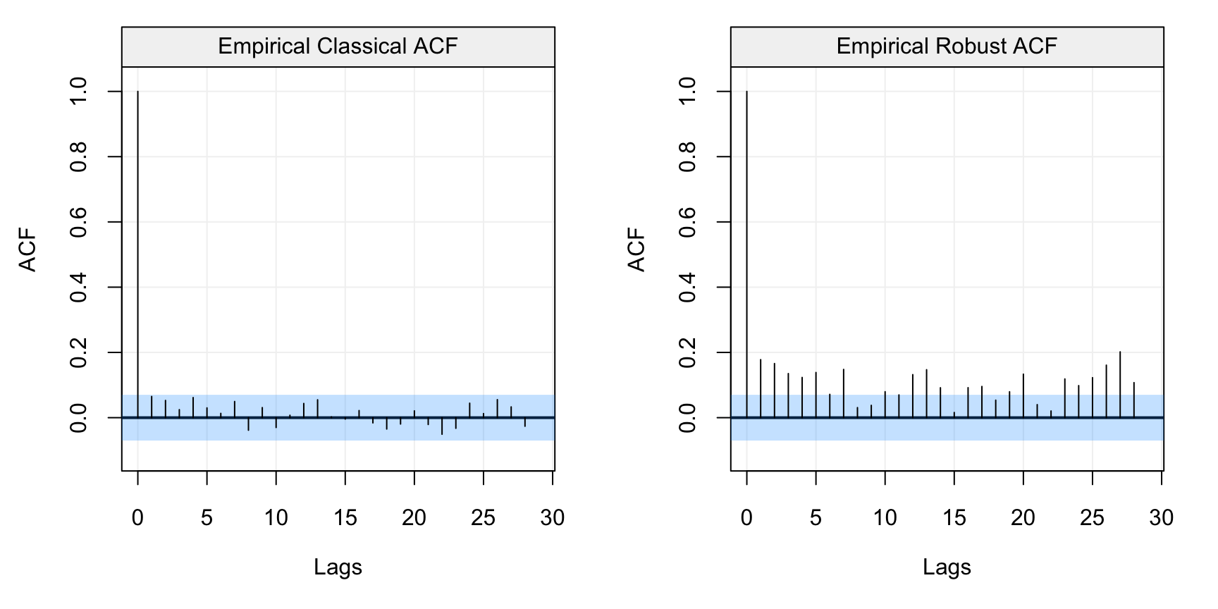
Figure 4.3: Standard (left) and robust (left) estimates of the ACF function on the monthly precipitation data (hydro)
As we had underlined in the previous chapter, the standard ACF estimates would suggest that there appears to be no correlation among lags and consequently, the WN model would be the most appropriate. However, the robust ACF estimates depict an entirely different picture where it can be seen that there appears to be a significant autocorrelation over different lags which exponentially decay. Although there appears to be some seasonality in the plot, we will assume that the correct model for this data is an AR(1) since that’s what hydrology theory suggests. Let us therefore estimate the parameters of this model by using a standard estimator (MLE) and a robust estimator (RGMWM). The estimates for the MLE are the following:
mle_hydro = estimate(AR(1), as.vector(hydro),  method = "mle", demean = TRUE)

# MLE Estimates
c(mle_hydro$mod$coef[1], mle_hydro$mod$sigma2)
## ar1
## 0.06497727 0.22205713From these estimates it would appear that the autocorrelation between lagged variables (i.e. lags of order 1) is extremely low and that (as suggested by the standard ACF plot) a WN model may be more appropriate. Considering the robust ACF however, it is possible that the MLE estimates may not be reliable in this setting. Hence, let us use the RGMWM to estimate the same parameters.
rgmwm_hydro = estimate(AR(1), hydro, method = "rgmwm")$mod$estimate

# RGMWM Estimates
t(rgmwm_hydro)
## AR SIGMA2
## Estimates 0.4048702 0.1065875In this case, we see how the autocorrelation between lagged values is much higher (0.4 compared to 0.06) indicating that there is a stronger dependence in the data than what is suggested by standard estimators. Moreover, the innovation variance is smaller compared to that of the MLE. This is also a known phenomenon when there’s contamination in the data since it leads to less dependence and more variability being detected by non-robust estimators. This estimate of the variance also has a considerable impact on forecast precision (as we’ll see in the next section).
A final applied example that highlights the (potential) difference between estimators according to the type of setting is given by the “Recruitment” data set (in the astsa library). This data refers to the presence of new fish in the population of the Pacific Ocean and is often linked to the currents and temperatures passing through the ocean. As for the previous data set, let us take a look at the data itself and then analyse the standard and robust estimations of the ACF.
# Format data
fish = gts(rec, start = 1950, freq = 12, unit_time = 'month', name_ts = 'Recruitment')

# Plot data
plot(fish)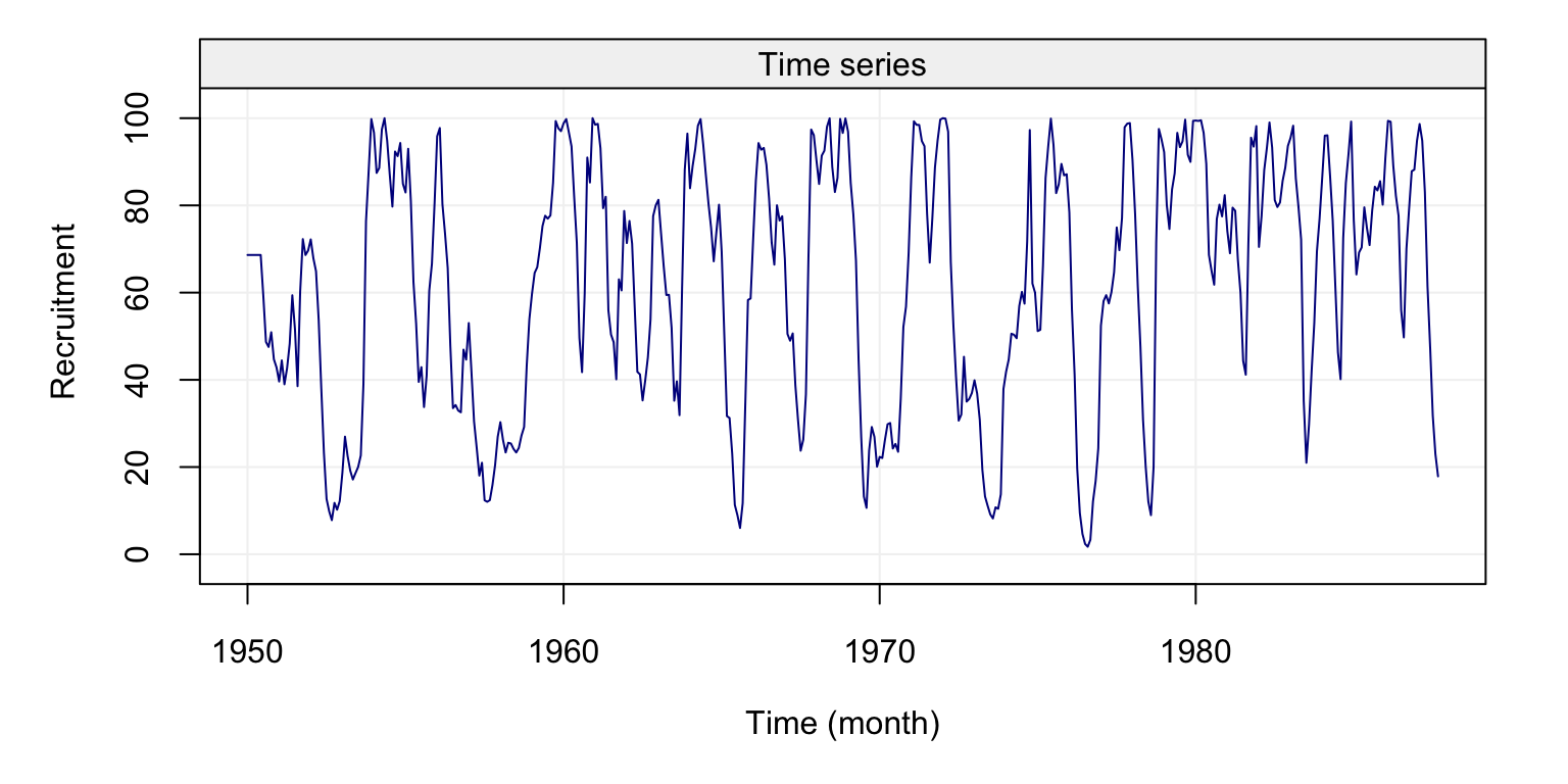
Figure 4.4: Plot of the time series on fish recruitment monthly data in the Pacific Ocean from 1950 to 1987
compare_acf(fish)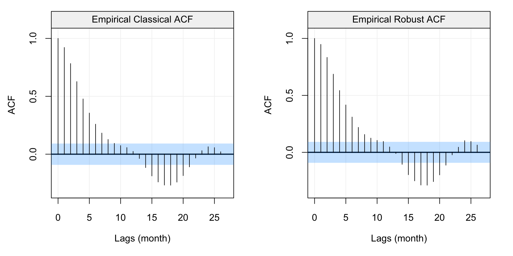
Figure 4.5: Standard (left) and robust (left) estimates of the ACF function on the monthly fish recruitment data (rec)
We can see that there appears to be a considerable dependence between the lagged variables which decays (in a similar way to the ACF of an AR(\(p\))). Also in this case we see a seasonality in the data but we won’t consider this for the purpose of this example. Given that there doesn’t appear to be any significant contamination in the data, let us consider the Yule-Walker and MLE estimators. The MLE highly depends on the assumed parametric distribution of the time series (i.e. usually Gaussian) and, if this is not respected, the resulting estimations could be unreliable. Hence, a first difference of the time series can often give an idea of the marginal distribution of the time series.
# Take first differencing of the recruitment data
diff_fish = gts(diff(rec), start = 1950, freq = 12, unit_time = 'month', name_ts = 'Recruitment')

# Plot first differencing of the recruitment data
plot(diff_fish)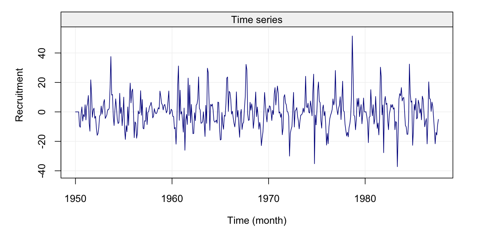
Figure 4.6: Plot of the first difference of the time series on fish recruitment monthly data in the Pacific Ocean from 1950 to 1987
From the plot we can see that observations appear to be collected around a constant value and fewer appear to be further from this value (as would be the case for a normal distribution). However, various of these “more extreme” observations appear to be quite frequent suggesting that the underlying distribution may have a heavier tail compared to the normal distribution. Let us compare the standard and robust ACF estimates of this new time series.
compare_acf(diff_fish)
Figure 4.7: Standard (left) and robust (left) estimates of the ACF function on the first difference of the monthly fish recruitment data (rec)
In this case we see that the patterns appear to be the same but the values between the standard and robust estimates are slightly (to moderately) different over different lags. This would suggest that there could be some contamination in the data or, in any case, that the normal assumption may not hold exactly. With this in mind, let us estimate an AR(2) model for this data using the Yule-Walker and MLE.
# MLE of Recruitment data
yw_fish = estimate(AR(2), rec, method = "yule-walker", demean = TRUE)

# MLE of Recruitment data
mle_fish = estimate(AR(2), rec, method = "mle", demean = TRUE)

# Compare estimates
# Yule-Walker Estimation
c(yw_fish$mod$coef[1], yw_fish$mod$sigma2)
## ar1
## 1.354069 89.717052# MLE Estimation
c(mle_fish$mod$coef[1], mle_fish$mod$sigma2)## ar1
## 1.351218 89.334361It can be seen that, in this setting, the two estimators deliver very similar results (at least in terms of the \(\phi_1\) and \(\phi_2\) coefficients). Indeed, there doesn’t appear to be a strong need for robust estimation and the choice of a standard estimator is justified by the will to obtain efficient estimations. The only slight difference between the two estimations is in the innovation variance parameter \(\sigma^2\) and this could be (evenutally) due to the normality assumption that the MLE estimator upholds in this case. If there is therefore a doubt on the fact that the Gaussian assumption does not hold for this data, then it is probably more convenient to use the Yule-Walker estimates.
Until now we have focussed on estimation based on an assumed model. However, how do we choose a model? How can we make inference on the models and their parameters? To perform all these tasks we will need to compute residuals (as, for example, in the linear regression framework). In order to obtain residuals, we need to be able to predict (forecast) values of the time series and, consequently, the next section focuses on forecasting time series.
4.2.3 Forecasting AR(p) Models
One of the most interesting aspects of time series analysis is to predict the future unobserved values based on the values that have been observed up to now. However, this is not possible if the underlying (parametric) model is unknown, thus in this section we assume, for purpose of illustration, that the time series \((X_t)\) is stationary and its model is known. In particular, we denote forecasts by \(X^{t}_{t+j}\), where \(t\) represents the time point from which we would like to make a forecast assuming we have an observed time series (e.g. \(\mathbf{X} = (X_{1}, X_{2}, \cdots , X_{t-1}, X_t)\)) and \(j\) represents the \(j^{th}\)-ahead future value we wish to predict. So, \(X^{t}_{t+1}\) represents a one-step-ahead prediction of \(X_{t+1}\) given data \((X_{1}, X_{2}, \cdots, X_{t-1}, X_{t})\).
Let us now focus on defining a prediction operator and, for this purpose, let us define the Mean Squared Prediction Error (MSPE) as follows:
\[\mathbb{E}[(X_{t+j} - X^{t}_{t+j})^2] .\] Intuitively, the MPSE measures the square distance (i.e. always positive) between the actual future values and the corresponding predictions. Ideally, we would want this measure to be equal to zero (meaning that we don’t make any prediction errors) but, if this is not possible, we would like to define a predictor that has the smallest MPSE among all possible predictors. The MPSE is not necessarily the best measure of prediction accuracy since, for example, it can be greatly affected by outliers or doesn’t take into account importance of positive or negative misspredictions (e.g. for risks in finance or insurance). Nevertheless, it is a good overall measure of forecast accuracy and the next theorem states what the best predictor is for this measure.
Theorem 4.1 (Minimum Mean Squared Error Predictor) Let us define \[X_{t + j}^t \equiv \mathbb{E}\left[ {{X_{t + j}}|{X_t}, \cdots ,{X_1}} \right], j > 0\]
Then \[\mathbb{E}\left[ {{{\left( {{X_{t + j}} - m\left( {{X_1}, \cdots ,{X_t}} \right)} \right)}^2}} \right] \ge \mathbb{E}\left[ {{{\left( {{X_{t + j}} - X_{t + j}^t} \right)}^2}} \right]\] for any function \(m(.)\).
The proof of this theorem can be found in Appendix A.2. Although this theorem defines the best possible predictor, there can be many functional forms for this operator. We first restrict our attention to the set of linear predictors defined as
\[X_{t+j}^t = \sum_{i=1}^t \alpha_i X_i,\] where \(\alpha_i \in \mathbb{R}\). It can be noticed, for example, that the \(\alpha_i\)’s are not always the same based on the values of \(t\) and \(j\) (i.e. it depends from which time point you want to predict and how far into the future). Another aspect to notice is that, if the time series model underlying the observed time series can be expressed in the form of a linear operator (e.g. a linear process), then we can derive a linear predictor from this framework.
Let us consider some examples to understand how these linear predictors can be delivered based on the AR(p) models studied this far. For this purpose, let us start with an AR(1) process.
Example 4.8 (Forecasting with an AR(1) model) The AR(1) model is defined as follows:
\[{X_t} = \phi {X_{t - 1}} + {W_t},\]
where \(W_t \sim WN(0, \sigma^2)\).
From here, the conditional expected mean and variance are given by
\[\begin{aligned} \mathbb{E}\left[ X_{t + j} | \Omega_t \right] &= \mathbb{E}[\phi X_{t+j-1} + W_{t+j}\,| \, \Omega_t ] \\ &= ... = {\phi ^j}{X_t} \\ \operatorname{var}\left[ {{X_{t + j}}} | \Omega_t \right] &= \left( {1 + {\phi ^2} + {\phi ^4} + \cdots + {\phi ^{2\left( {j - 1} \right)}}} \right){\sigma ^2} \\ \end{aligned} \]
Within this derivation, it is important to remember that
\[\begin{aligned} \mathop {\lim }\limits_{j \to \infty } \mathbb{E}\left[ {{X_{t + j}}} | \Omega_t \right] &= \mathbb{E}\left[ {{X_t}} \right] = 0 \\ \mathop {\lim }\limits_{j \to \infty } \operatorname{var}_t\left[ {{X_{t + j}}} | \Omega_t \right] &= \operatorname{var} \left( {{X_t}} \right) = \frac{{{\sigma ^2}}}{{1 - {\phi ^2}}} \end{aligned} \]
From these last results we see that the forecast for an AR(1) process is “mean-reverting” since in general we have that the AR(1) can be written with respect to the mean \(\mu\) as follows
\[(X_t - \mu) = \phi (X_{t-1} - \mu) + W_t,\]
which gives
\[X_t = \mu + \phi (X_{t-1} - \mu) + W_t,\]
and consequently
\[\begin{aligned} \mathbb{E}[X_{t+j} | \Omega_t] &= \mu + \mathbb{E}[(X_{t+j} - \mu) | \Omega_t] \\ &= \mu + \phi^j(X_t - \mu), \end{aligned} \]
which tends to \(\mu\) as \(j \to \infty\)Let us now consider a more complicated model, i.e. an AR(2) model.
Example 4.9 (Forecasting with an AR(2) model) Consider an AR(2) process defined as follows:
\[{X_t} = {\phi _1}{X_{t - 1}} + {\phi _2}{X_{t - 2}} + {W_t},\]
where \(W_t \sim WN(0, \sigma^2)\).
Based on this process we are able to find the predictor for each j-step ahead prediction using the following approach:
\[\begin{aligned} \mathbb{E}\left[ {{X_{t + 1}}} | \Omega_t \right] &= {\phi _1}{X_t} + {\phi _2}{X_{t - 1}} \\ \mathbb{E}\left[ {{X_{t + 2}}} | \Omega_t \right] &= \mathbb{E}\left[ {{\phi _1}{X_{t + 1}} + {\phi _2}{X_t}} | \Omega_t \right] = {\phi _1} \mathbb{E}\left[ {{X_{t + 1}}} | \Omega_t \right] + {\phi _2}{X_t} \\ &= {\phi _1}\left( {{\phi _1}{X_t} + {\phi _2}{X_{t - 1}}} \right) + {\phi _2}{X_t} \\ &= \left( {\phi _1^2 + {\phi _2}} \right){X_t} + {\phi _1}{\phi _2}{X_{t - 1}}. \\ \end{aligned} \]
Having seen how to build a forecast for an AR(1), let us now generalise this method to an AR(p) using matrix notation.
Example 4.10 (Forecasting with an AR(p) model) Consider AR(p) process defined as:
\[{X_t} = {\phi _1}{X_{t - 1}} + {\phi _2}{X_{t - 2}} + \cdots + {\phi _p}{X_{t - p}} + {W_t},\]
where \(W_t \sim WN(0, \sigma^2_W)\).
The process can be rearranged into matrix form as follows:
\[\begin{aligned} \underbrace {\left[ {\begin{array}{*{20}{c}} {{X_t}} \\ \vdots \\ \vdots \\ {{X_{t - p + 1}}} \end{array}} \right]}_{{Y_t}} &= \underbrace {\left[ {\begin{array}{*{20}{c}} {{\phi _1}}& \cdots &{}&{{\phi _p}} \\ {}&{}&{}&0 \\ {}&{{I_{p - 1}}}&{}& \vdots \\ {}&{}&{}&0 \end{array}} \right]}_A\underbrace {\left[ {\begin{array}{*{20}{c}} {{X_{t - 1}}} \\ \vdots \\ \vdots \\ {{X_{t - p}}} \end{array}} \right]}_{{Y_{t - 1}}} + \underbrace {\left[ {\begin{array}{*{20}{c}} 1 \\ 0 \\ \vdots \\ 0 \end{array}} \right]}_C{W_t} \\ {Y_t} &= A{Y_{t - 1}} + C{W_t} \end{aligned}\]
From here, the conditional expectation and variance can be computed as follows:
\[\begin{aligned} {E}\left[ {{Y_{t + j}}} | \Omega_t \right] &= {E}\left[ {A{Y_{t + j - 1}} + C{W_{t + j}}} | \Omega_t\right] = {E}\left[ {A{Y_{t + j - 1}}} | \Omega_t \right] + \underbrace {{E}\left[ {C{W_{t + j}}} | \Omega_t \right]}_{ = 0} \\ &= {E}\left[ {A\left( {A{Y_{t + j - 2}} + C{W_{t + j - 1}}} \right)} | \Omega_t \right] = {E}\left[ {{A^2}{Y_{t + j - 2}}} | \Omega_t\right] = {A^j}{Y_t} \\ {\operatorname{var}}\left[ {{Y_{t + j}}} | | \Omega_t\right] &= {\operatorname{var}}\left[ {A{Y_{t + j - 1}} + C{W_{t + j}}} | \Omega_t \right] \\ &= {\sigma ^2}C{C^T} + {\operatorname{var}}\left[ {A{Y_{t + j - 1}}} | \Omega_t \right] = {\sigma ^2}A{\operatorname{var}}\left[ {{Y_{t + j - 1}}} | \Omega_t \right]{A^T} \\ &= {\sigma ^2}C{C^T} + {\sigma ^2}AC{C^T}A + {\sigma ^2}{A^2}{\operatorname{var}}\left[ {{Y_{t + j - 2}}} | \Omega_t \right]{\left( {{A^2}} \right)^T} \\ &= {\sigma ^2}\sum\limits_{k = 0}^{j - 1} {{A^k}C{C^T}{{\left( {{A^K}} \right)}^T}} \\ \end{aligned} \]
Considering the recursive pattern coming from the expressions of the conditional expectation and variance, the predictions can be obtained via the following recursive formulation: \[\begin{aligned} {E}\left[ {{Y_{t + j}}} | \Omega_t \right] &= A{E}\left[ {{Y_{t + j - 1}}} | \Omega_t\right] \\ {\operatorname{var}}\left[ {{Y_{t + j}}} | \Omega_t \right] &= {\sigma ^2}C{C^T} + A{\operatorname{var}}\left[ {{Y_{t + j - 1}}} | \Omega_t \right]{A^T} \\ \end{aligned} \]With this recursive expression we can now compute the conditional expectation and variance of different AR(p) models. Let us therefore revisit the previous AR(2) example using this recursive formula.
Example 4.11 (Forecasting with an AR(2) in Matrix Form) We can rewrite our previous example of the predictions for an AR(2) process as follows
\[\begin{aligned} \underbrace {\left[ {\begin{array}{*{20}{c}} {{X_t}} \\ {{X_{t - 1}}} \end{array}} \right]}_{{Y_t}} &= \underbrace {\left[ {\begin{array}{*{20}{c}} {{\phi _1}}&{{\phi _2}} \\ 1&0 \end{array}} \right]}_A\underbrace {\left[ {\begin{array}{*{20}{c}} {{X_{t - 1}}} \\ {{X_{t - 2}}} \end{array}} \right]}_{{Y_{t - 1}}} + \underbrace {\left[ {\begin{array}{*{20}{c}} 1 \\ 0 \end{array}} \right]}_C{W_t} \\ {Y_t} &= A{Y_{t - 1}} + C{W_t} \end{aligned}\]
Then, we are able to calculate the prediction as
\[\begin{aligned} {E}\left[ {{Y_{t + 2}}} | \Omega_t \right] &= {A^2}{Y_t} = \left[ {\begin{array}{*{20}{c}} {{\phi _1}}&{{\phi _2}} \\ 1&0 \end{array}} \right]\left[ {\begin{array}{*{20}{c}} {{\phi _1}}&{{\phi _2}} \\ 1&0 \end{array}} \right]\left[ {\begin{array}{*{20}{c}} {{X_t}} \\ {{X_{t - 1}}} \end{array}} \right] \hfill \\ &= \left[ {\begin{array}{*{20}{c}} {\phi _1^2 + {\phi _2}}&{{\phi _1}{\phi _2}} \\ {{\phi _1}}&{{\phi _2}} \end{array}} \right]\left[ {\begin{array}{*{20}{c}} {{X_t}} \\ {{X_{t - 1}}} \end{array}} \right] = \left[ {\begin{array}{*{20}{c}} {\left( {\phi _1^2 + {\phi _2}} \right){X_t} + {\phi _1}{\phi _2}{X_{t - 1}}} \\ {{\phi _1}{X_t} + {\phi _2}{X_{t - 1}}} \end{array}} \right] \hfill \\ \end{aligned} \]The above examples have given insight as to how to compute predictors for the AR(p) models that we have studied this far. Let us now observe the consequences of using such an approach to predict future values from these models. For this purpose, using the recursive formulation seen in the examples above we perform a simulation study where, for a fixed set of parameters, we make 5000 predictions from an observed time series and predict 50 values ahead into the future. The known parameters for the AR(2) process we use for the simulation study are \(\phi _1 = 0.75\), \(\phi _2 = 0.2\) and \(\sigma^2 = 1\). The figure below shows the distribution of these predictions starting from the last observation \(T = 200\).
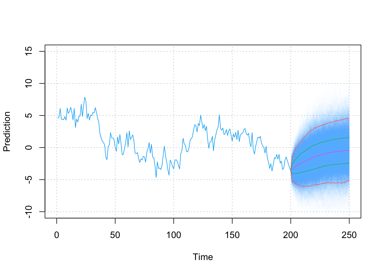
Figure 4.8: Values of the AR(2) predictions with the pink line being the median prediction, red and green lines are respectively 95% and 75% Confidence intervals.
It can be observed that, as hinted by the expressions for the variance of the predictions (in the examples above), the variability of the predictions increases as we try to predict further into the future.
Having now defined the basic concepts for forecasting of time series we can now start another topic of considerable importance for time series analysis. Indeed, the whole discussion on prediction is not only important to derive forecasts for future values of the phenomena one may be interested in, but also in understanding how well a model explains (and predicts) an observed time series. In fact, predictions allow to deliver residuals within the time series setting and, based on these residuals, we can obtain different inference and diagnostic tools.
Given the knowledge on predictions seen above, residuals can be computed as
\[r_{t+j} = X_{t+j} - \hat{X}_{t+j},\] where \(\hat{X}_{t+j}\) represents an estimator of the conditional expectation \(E[X_{t+j} | \Omega_{t}]\). The latter quantity will depend on the model underlying the time series and, assuming we know the true model, we could use the true parameters to obtain a value for this expectation. However, in an applied setting it is improbable that we know the true parameters and therefore \(\hat{X}_{t+j}\) can be obtained by estimating the parameters (as seen in the previous sections) and then plugging thmem into the expression of \(E[X_{t+j} | \Omega_{t}]\).
4.3 Diagnostic Tools for Time Series
The standard approach to understanding how well a model fits the data is analysing the residuals (e.g. linear regression). The same approach can be taken for time series analysis where, given our knowledge on forecasts from the previous section, we can now deliver residuals. The first step (and possibly the most important) is to use visual tools to check the residuals and also the original time series. Below is a figure that collects different diagnostic tools for time series analysis and is applied to a simulated AR(1) process of length \(T = 100\).
set.seed(333)
true_model = AR(phi = 0.8, sigma2 = 1)
Xt = gen_gts(n = 100, model = true_model)
model = estimate(AR(1), Xt, demean = FALSE)
check(model = model)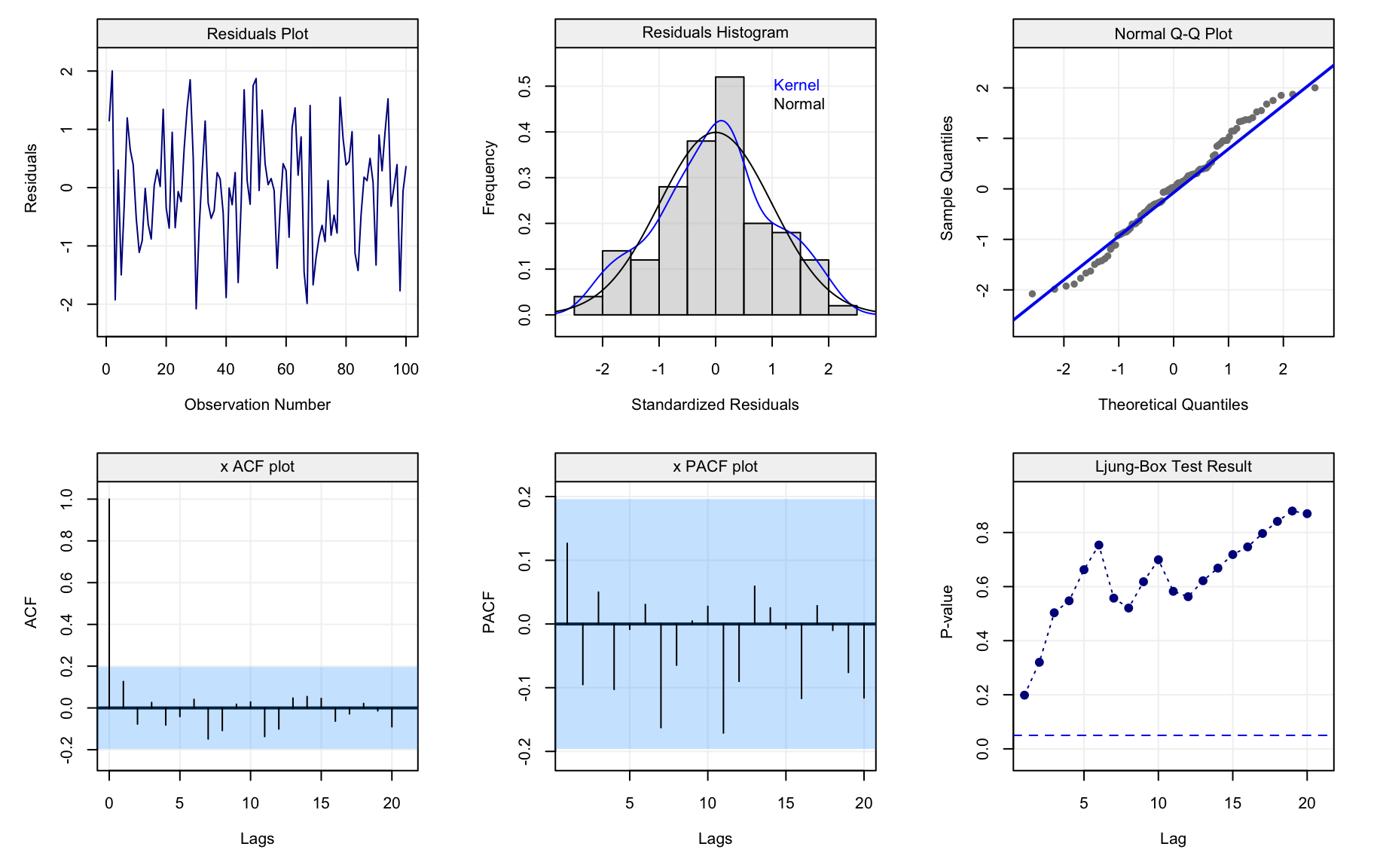
(#fig:diagnostic_plot)Ljung-Box test p-values for the residuals of the fitted AR(1) model over lags \(h = 1, ...., 20\).
All plots refer to the residuals of the model-fit and aim at visually assessing whether the fitted time series model captures the dependence structure in the data. The first row contains plots that can be interpreted in the same manner as the residuals from a linear regression. The first plot simply represents the residuals over time and should show if there is any presence of trends, seasonality or heteroskedasticity. The second plot gives a histogram (and smoothed histrogram called a kernel) of the residuals which should be centered in zero and (possibly) have an approximate normal distribution. The latter hypothesis can also be checked using the third plot which consists in a Normal quantile-quantile plot and the residuals should lie on (or close to) the diagonal line representing correspondance between the distributions.
The first plot in the second row in the above figureshows the estimated ACF. It can be seen how the estimated autocorrelations all lie within the blue shaded area representing the confidence intervals. The second plot represents the Partial AutoCorrelation Function (PACF) and is another tool that will be investigated further on. In the meantime, suffice it to say that this tool can be interpreted as a different version of the ACF which measures autocorrelation conditionally on the previous lags (in some sense, it measures the direct impact of \(X_t\) on \(X{t+h}\) removing the influence of all observations inbetween). In this case, we see that also the estimated PACF lies within the confidence intervals and, along with the intepretation of the ACF, we can state that the model appears to fit the time series reasonably well since the residuals can be considered as following a white noise process. Finally, the last plot visualises the “Ljung-Box Test” (which is a type of Portmanteau test) that tests whether the autocorrelation of the residuals at a set of lags is different from zero. The plot represents the p-value of this test at the different lags and also shows a dashed line representing the common significance level of \(\alpha = 0.05\). If the modelling has done a good job, all p-values should be larger than this level. In this case, using the latter level, we can see that the autocorrelations for the residuals appear to be non-significant and therefore fitting an AR(1) model to the time series (which is the true model in this example) appears to do a reasonably good job.
4.3.1 The Partial AutoCorrelation Function (PACF)
Before further discussing these diagnostic tools, let us focus a little more on the PACF mentioned earlier. As briefly highlighted above, this function measures the degree of linear correlation between two lagged observations by removing the effect of the observations in the intermediate lags. For example, let us assume we have three correlated variables \(X\), \(Y\) and \(Z\) and we wish to find the direct correlation between \(X\) and \(Y\): we can apply a linear regression of \(X\) on \(Z\) (to obtain \(\hat{X}\)) and \(Y\) on \(Z\) (to obtain \(\hat{Y}\)) and thereby compute \(corr(\hat{X}, \hat{Y})\) which represents the partial autocorrelation. In this manner, the effect of \(Z\) on the correlation between \(X\) and \(Y\) is removed. Considering the variables as being indexed by time (i.e. a time series), we can therefore define the following quantities \[\hat{X}_{t+h} = \beta_1 X_{t+h-1} + \beta_2 X_{t+h-2} + ... + \beta_{h-1} X_{t+1},\] and
\[\hat{X}_{t} = \beta_1 X_{t+1} + \beta_2 X_{t+2} + ... + \beta_{h-1} X_{t+h-1},\] which represent the regressions of \(X_{t+h}\) and \(X_t\) on all intermediate observations. With these defintions, let us more formally define the PACF.
Therefore, the PACF is not defined at lag zero while it is the same as the ACF at the first lag since there are no intermediate observations. The defintion of this function is important for different reasons. Firstly, as mentioned earlier, we have an asymptotic distribution for the estimator of the PACF which allows us to deliver confidence intervals as for the ACF. Indeed, representing the empirical PACF along with its confidence intervals can provide a further tool to make sure that the residuals of a model fit can be considered as being white noise. The latter is a reasonable hypothesis if both the empirical ACF and PACF lie within the confidence intervals indicating that there is no significant correlation between lagged variables. Let us focus on the empirical PACF of the residuals we saw earlier in the diagnostic plot.
residuals = model$mod$residuals
plot(auto_corr(residuals, pacf = TRUE))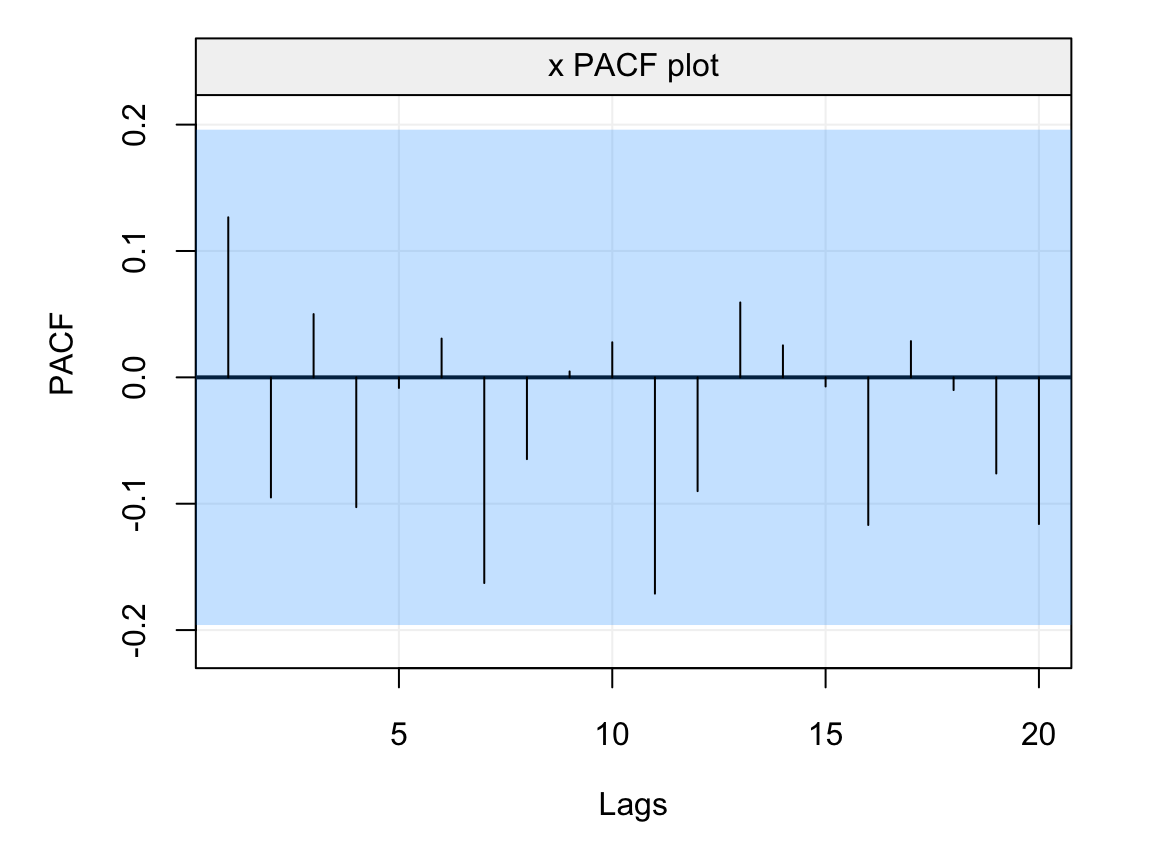
Figure 4.9: Empirical PACF on the residuals of the AR(1) model fitted to the simulated time series generated from an AR(1) process.
From the plot we see that the estimated PACF at all lags lies within the blue shaded area representing the 95% confidence intervals indicating that the residuals don’t appear to have any form of direct autocorrelation over lags and, hence, that they can be considered as white noise. In addition to delivering a tool to analyse the residuals of a model fit, the PACF is especially useful for diagnostic purposes in order to detect the possible models that have generated an observed time series. With respect to the class of models studied this far (i.e. AR(\(p\)) models), the PACF can give important insight to the order of the AR(\(p\)) model, more specifically the value of \(p\). Indeed, the ACF of an AR(\(p\)) model tends to decrease in a sinusoidal fashion and exponetially fast to zero as the lag \(h\) increases thereby giving a hint that the underlying model belongs to the AR(\(p\)) family. However, aside from hinting to the fact that the model belongs to the family of AR(\(p\)) models, the latter function tends to be less informative with respect to which AR(\(p\)) model (i.e. which value of \(p\)) is best suited for the observed time series. The PACF on the other hand is non-zero for the first \(p\) lags and then becomes zero for \(h > p\), therefore it can give an important indication with respect to which order should be considered to best model the time series.
With the above discussion in mind, let us consider some examples where we study the theoretical ACF and PACF of different AR(\(p\)) models. The first is an AR(1) model with parameter \(\phi = 0.95\) and its ACF and PACF are shown below.
par(mfrow = c(1, 2))
plot(theo_acf(ar = 0.95, ma = NULL))
plot(theo_pacf(ar = 0.95, ma = NULL))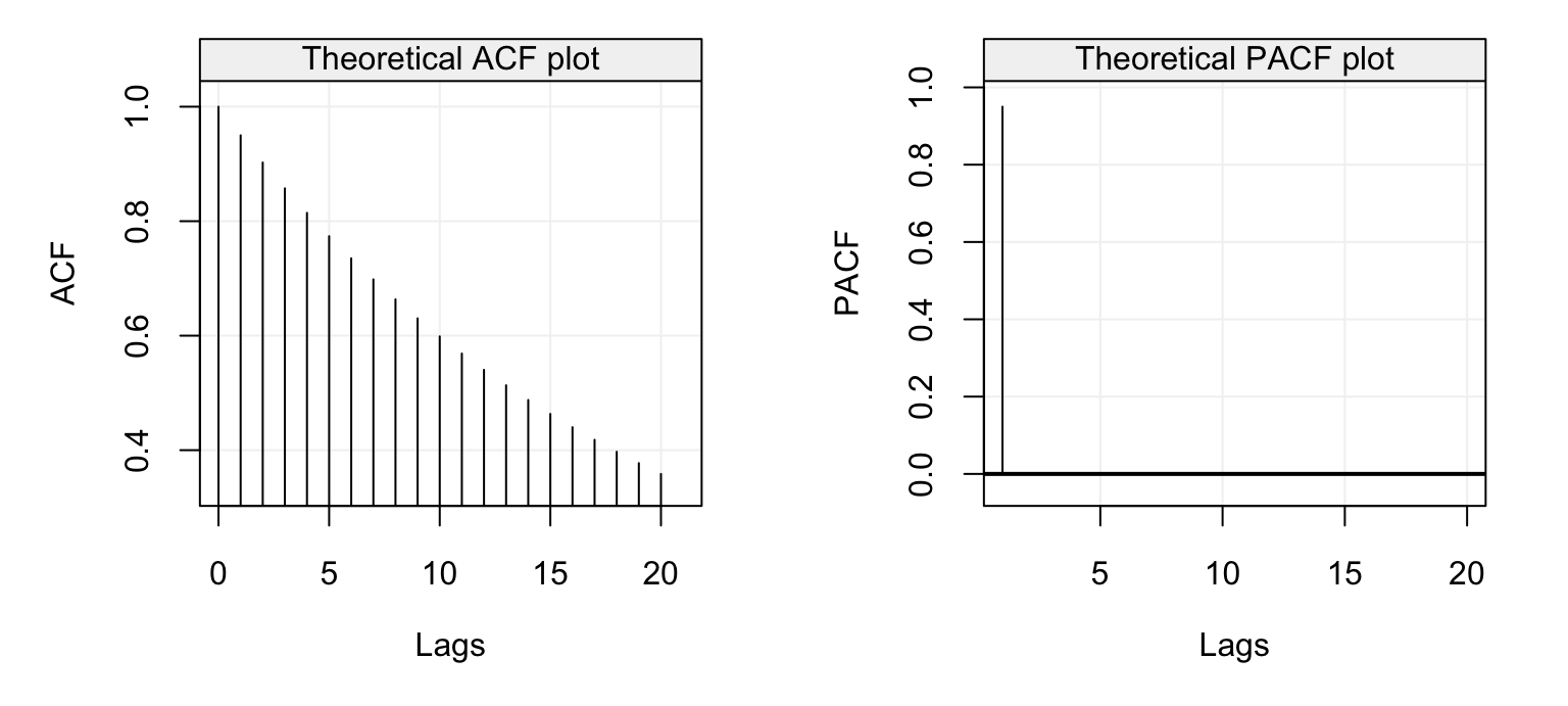
Figure 4.10: Theoretical ACF (left) and PACF (right) of an AR(1) model with parameter \(\phi = 0.95\).
We can see that the ACF decreases exponentially fast as we would expect for an AR(p) model while the PACF has the same values of the ACF at lag 1 (which is always the case) and is zero for \(h > 1\). The latter therefore indicates the order \(p\) of the AR(\(p\)) model which in this case is \(p=1\). Let us now consider the following models as further examples:
\[X_t = 0.5 X_{t-1} + 0.25 X_{t-2} + 0.125 X_{t-3} + W_t\]
and
\[X_t = -0.1 X_{t-2} -0.1 X_{t-4} + 0.6 X_{t-5} + W_t.\]
The first model is an AR(3) model with positive coefficients while the second is an AR(5) model where \(\phi_1 = \phi_3 = 0\). The ACF and PACF of the first AR(3) model is shown below.
par(mfrow = c(1, 2))
plot(theo_acf(ar = c(0.5, 0.25, 0.125), ma = NULL))
plot(theo_pacf(ar = c(0.5, 0.25, 0.125), ma = NULL))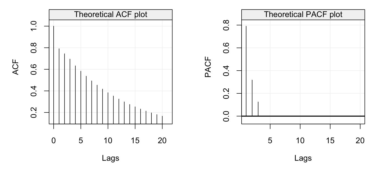
Figure 4.11: Theoretical ACF (left) and PACF (right) of an AR(3) model with parameters \(\phi_1 = 0.95\), \(\phi_2 = 0.25\) and \(\phi_3 = 0.125\).
Again, we see that the ACF decreases exponentially and also the PACF plot shows a steady decrease until it becomes zero for \(h > 3\). This is because the values of \(\phi_i\) are all positive and decreasing as well. Let us now consider the second model (the AR(5) model) whose ACF and PACF plots are represented below.
par(mfrow = c(1, 2))
plot(theo_acf(ar = c(0, -0.1, 0, -0.1, 0.6), ma = NULL))
plot(theo_pacf(ar = c(0, -0.1, 0, -0.1, 0.6), ma = NULL))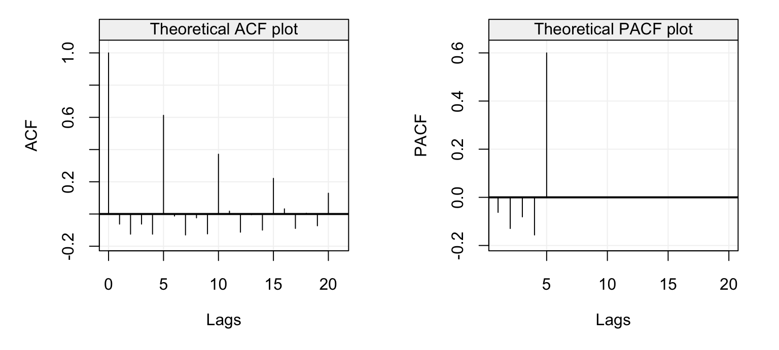
Figure 4.12: Theoretical ACF (left) and PACF (right) of an AR(4) model with parameters \(\phi_1 = 0\), \(\phi_2 = -0.1\), \(\phi_3 = 0\) and \(\phi_4 = 0\).
In this case we see that the ACF has a sinusoidal-like behaviour where the values of \(\phi_1 = \phi_3 = 0\) and the negative \(\phi_2 = \phi_4 = -0.1\) values deliver this alternating ACF form which nevertheless decreases as \(h\) increases. These values deliver the PACF plot on the right which is negative for the first lags and is greatly positive at \(h=5\) only to become zero for \(h > 5\).
These examples therefore give us further insight as to how to interpret the empirical (or estimated) versions of these functions. For this reason, let us study the empirical ACF and PACF of some real time series, the first of which is the data representing the natural logarithm of the annual number of Lynx trappings in Canada between 1821 and 1934. The time series is represented below.
lynx_gts = gts(log(lynx), start = 1821, data_name = "Lynx Trappings", unit_time = "year", name_ts = "Trappings")
plot(lynx_gts)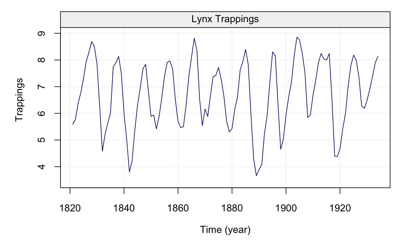
Figure 4.13: Time series of annual number of lynx data trappings in Canada between 1821 and 1934.
We can see that there appears to be a seasonal trend within the data but let us ignore this for the moment and check the ACF and PACF plots below.
corr_analysis(lynx_gts)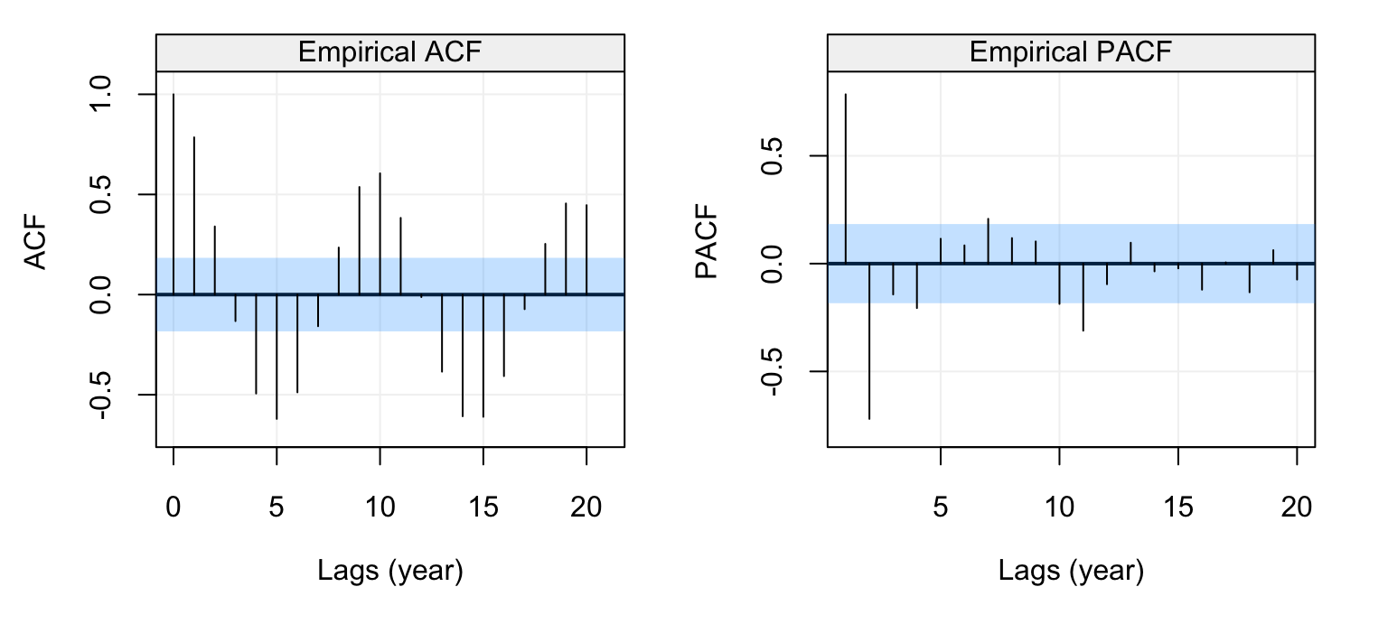
Figure 4.14: Empirical ACF (left) and PACF (right) of the lynx time series data.
The seasonal behaviour also appears in the ACF plot but we see that it decreases in a sinusoidal fashion as the lag increases hinting that an AR(p) model could be a potential candidate for the time series. Looking at the PACF plot on the right we can see that a few partial autocorrelations appear to be significant up to lag \(h=11\). Therefore an AR(11) model could be a possibly good candidate to explain (and predict) this time series.
4.3.2 Portmanteau Tests
In a similar manner to using the ACF and PACF confidence intervals to understand if the residuals can be considered as white noise, other statistical tests exist to determine if the autocorrelations can be considered as being significant or not. Indeed, the 95% confidence intervals can be extremely useful in detecting significant (partial) autocorrelations but they cannot be considered as an overall test for white noise since (aside from being asymptotic and therefore approximate) they do not consider the multiple testing hypothesis implied by them (i.e. if we’re testing all lags, the actual level of significance should be modified in order to bound type I errors). For this reason, Portmanteau tests have been proposed in order to deliver an overall test that jointly considers a set of lags and determines whether their autocorrelation is significantly different from zero (i.e. whether the residuals can be considered white noise or not).
One of the most popular Portmanteau tests is the Ljung-Box test whose statistic is defined as follows:
\[Q_h = T(T+2) \sum_{j=1}^{h} \frac{\hat{\rho}_j^2}{T - j},\] where \(h\) represents the maximum lag of the set of lags for which we wish to test for serial autocorrelation (i.e. from lag 1 to lag \(h\)). Under the null hypothesis \(Q_h \sim \chi_h^2\) since asymptotically \(\hat{\rho}_j \sim \mathcal{N}\left(0, \frac{1}{T}\right)\) under the null and therefore the statistic is proportional to the sum of squared standard normal variables. The last plot of Figure @ref(fig:diagnostic_plot) can therefore be better interpreted under this framework and is reproduced below.
lb_test = diag_ljungbox(as.numeric(residuals), order = 0, stop_lag = 20, stdres = FALSE, plot = TRUE)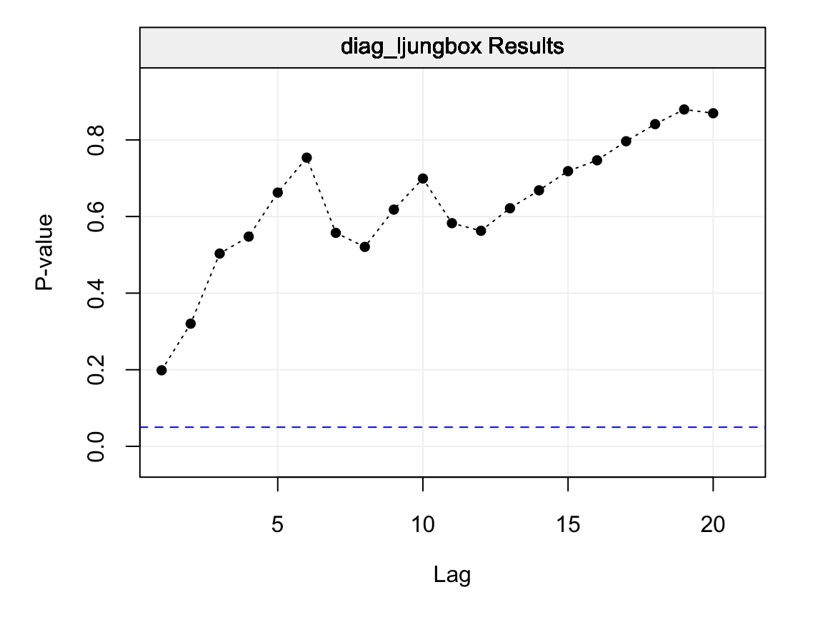
Figure 4.15: Ljung-Box p-values for lags \(h = 1,...,20\) on the residuals of the fitted AR(1) model.
Each p-value represented in the plot above is therefore the p-value for the considered maximum lag. Therefore the first p-value (at lag 1) is the p-value for the null hypothesis that all lags up to lag 1 are equal to zero, the second is for the null hypothesis that all lags up to lag 2 are equal to zero and so on. Hence, each p-value represents a global test on the autocorrelations up to the considered maximum lag \(h\) and delivers additional information regarding the dependence structure within the residuals. In this case, as interpreted earlier, all p-values are larger than the \(\alpha = 0.05\) level and is an additional indication that the residuals follow a white noise process (and that the fitted model appears to well describe the observed time series).
There are other Portmanteau tests with different advantages (and disadvantages) over the Ljung-Box test but these are beyond the scope of this textbook.
4.4 Inference for AR(p) Models
For all the above methods, it would be necessary to understand how “precise” their estimates are. To do so we would need to obtain confidence intervals for these estimates and this can be done mainly in two manners:
- using the asymptotic distribution of the parameter estimates;
- using parametric bootstrap.
The first approach consists in using the asymptotic distribution of the estimators presented earlier to deliver approximations of the confidence intervals which get better as the length of the observed time series increases. Hence, if for example we wanted to find a 95% confidence interval for the parameter \(\phi\), we would use the quantiles of the normal distribution (given that all methods presented earlier present this asymptotic distribution). However, this approach can present some drawbacks, one of which its behaviour when the parameters are close to the boundaries of the parameter space. Suppose we consider a realization of length \(T = 100\) of the following AR(1) model:
\[X_t = 0.96 X_{t-1} + W_t, \;\;\;\; W_t \sim \mathcal{N}(0,1),\]
which is represented in Figure 4.16
set.seed(55)
x = gen_gts(n = 100, AR1(0.96, 1))
plot(x)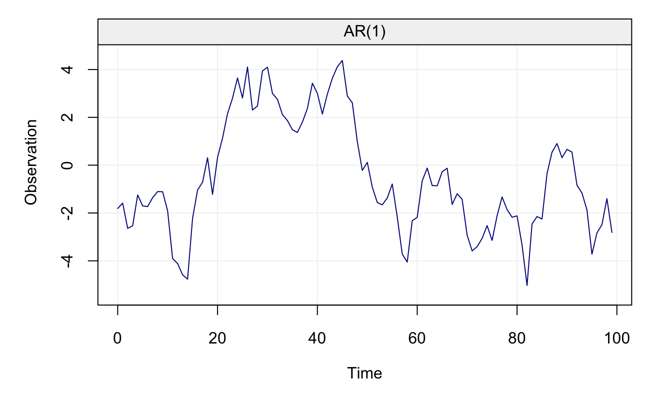
Figure 4.16: AR(1) with \(\phi\) close to parameter bound
It can be seen that the parameter \(\phi = 0.96\) respects the condition for stationarity (i.e.\(\left| \phi \right| < 1\)) but is very close to its boundary. Using the MLE, we first estimate the parameters and then compute confidence intervals for \(\phi\) using the asymptotic normal distribution.
# Compute the parameter estimates using MLE
fit.ML = estimate(AR(1), x, demean = FALSE)
c("phi" = fit.ML$mod$coef[1], "sigma2" = sqrt(fit.ML$mod$sigma2))
## phi.ar1 sigma2
## 0.9740770 0.8538777# Construct asymptotic confidence interval for phi
fit.ML$mod$coef[1] + c(-1,1)*1.96*as.numeric(sqrt(fit.ML$mod$var.coef))## [1] 0.9393414 1.0088127## Fitted model: AR(1)
##
## Estimated parameters:
## Model Information:
## Estimates
## AR 0.9864031
## SIGMA2 0.7644610
##
## * The initial values of the parameters used in the minimization of the GMWM objective function
## were generated by the program underneath seed: 1337.
##
## 95 % confidence intervals:
## Estimates CI Low CI High SE
## AR 0.9864031 0.8688122 1.054986 0.05659269
## SIGMA2 0.7644610 0.5565939 0.926104 0.11232308From the estimation summary, we can notice that the MLE confidence intervals contain values that would make the AR(1) non-stationary (i.e. values of \(\phi\) larger than 1). However, these confidence intervals are based on the (asymptotic) distributions of \(\hat{\phi}\) which are shown in Figure 4.17 along with those based on the GMWM estimator.
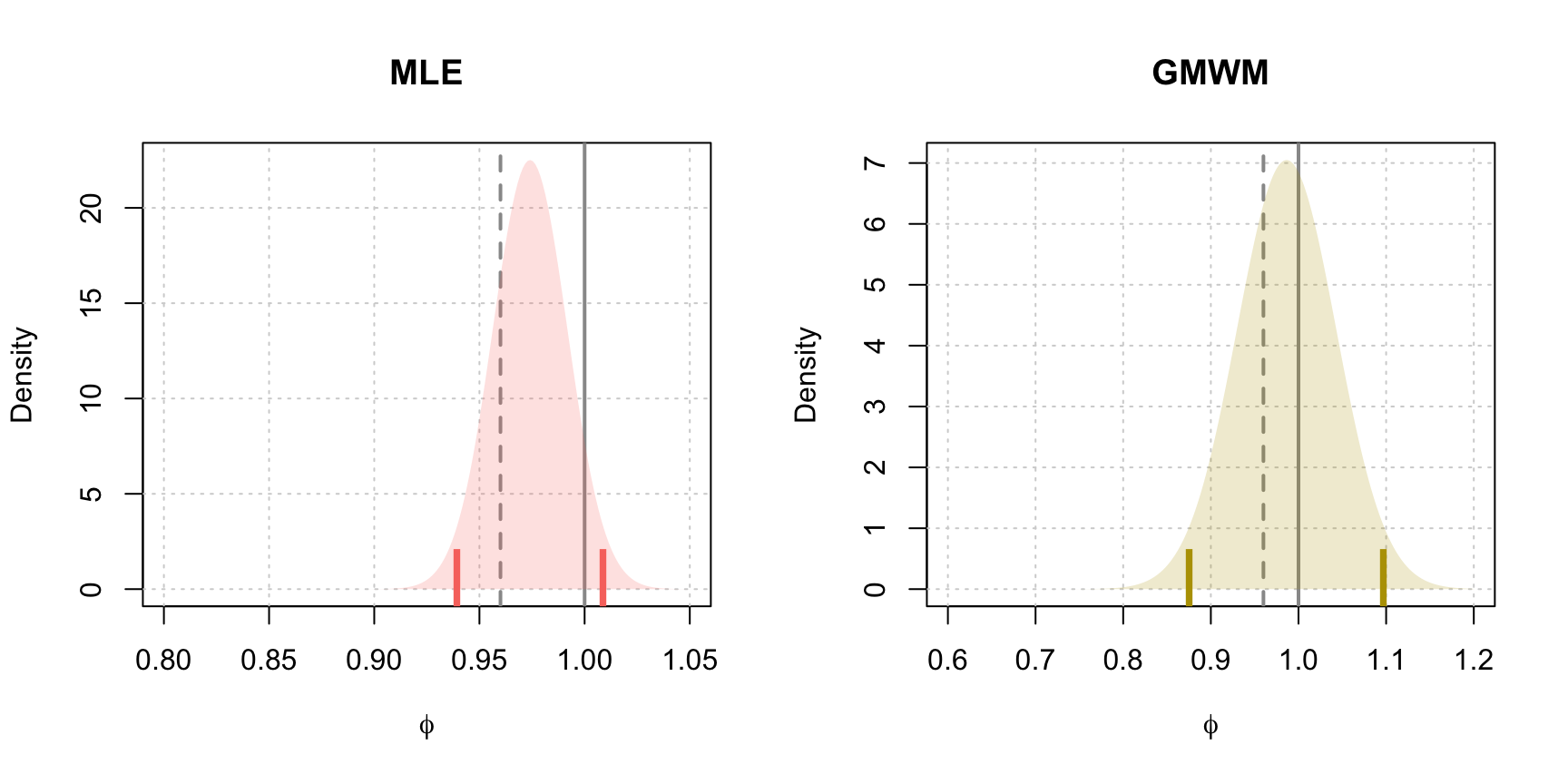
Figure 4.17: Estimated asymptotic distribution of \(\hat{\phi}\) for MLE and GMWM parameter estimates. The dashed vertical line represents the true value of \(\phi\), the solid line denotes the upper bound of the parameter space for \(\phi\) and the vertical ticks represent the limits of the 95% confidence intervals for both methods.
Therefore, if we estimate a stationary AR(1) model, it would be convenient to have more “realistic” confidence intervals that give limits for a stationary AR(1) model. A viable solution for this purpose is to use parametric bootstrap. Indeed, parametric bootstrap takes the estimated parameter values and uses them in order to simulate from the assumed model (an AR(1) process in this case). For each simulation, the parameters are estimated and stored in order to obtain an empirical (finite sample) distribution of the estimators. Based on this distribution it is consequently possible to find the \(\alpha/2\) and \(1-\alpha/2\) empirical quantiles thereby delivering confidence intervals that should not suffer from boundary problems (since the estimation procedure looks for solutions within the admissable regions). The code below gives an example of how this confidence interval is built based on the same estimation procedure but using parametric bootstrap (using \(B = 10,000\) bootstrap replicates).
# Number of Iterations
B = 10000

# Set up storage for results
est.phi.gmwm = rep(NA,B)
est.phi.ML = rep(NA,B)

# Model generation statements
model.gmwm = AR(phi = c(fit.gmwm$mod$estimate[1]), sigma2 = c(fit.gmwm$mod$estimate[2]))
model.mle = AR(phi = c(fit.ML$mod$coef), sigma2 = c(fit.ML$mod$sigma2))

# Begin bootstrap
for(i in seq_len(B)){

  # Set seed for reproducibility
  set.seed(B + i)

  # Generate process under MLE parameter estimate
  x.star = gen_gts(100, model.mle)

  # Attempt to estimate phi by employing a try
  est.phi.ML[i] = tryCatch(estimate(AR(1), x.star, demean = FALSE)$mod$coef,
                           error = function(e) NA)

  # Generate process under GMWM parameter estimate
  x.star = gen_gts(100, model.gmwm)
  est.phi.gmwm[i] = estimate(AR(1), x.star, method = "gmwm")$mod$estimate[1]
}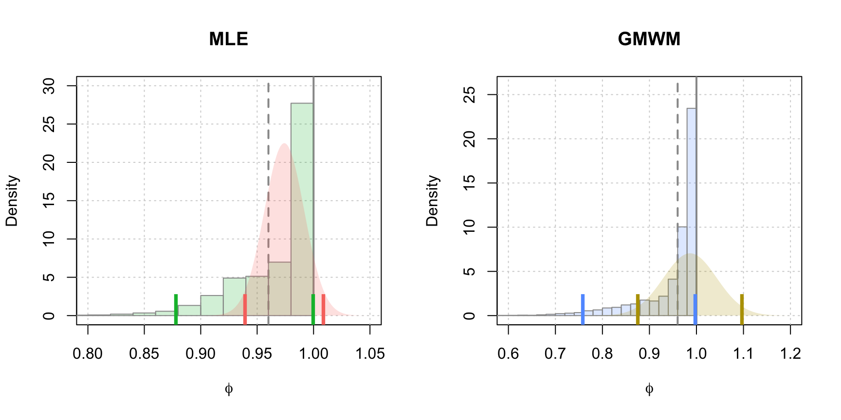
Figure 4.18: Parametric bootstrap distributions of \(\hat{\phi}\) for the MLE and GMWM parameter estimates. The histograms represent the empirical distributions resulting from the parametric bootstrap while the continuous densities represent the estimated asymptotic distributions. The vertical line represents the true value of \(\phi\), the dark solid lines represent the upper bound of the parameter space for \(\phi\) and the vertical ticks represent the limits of the 95% confidence intervals for the asymptotic distributions (red and gold) and the empirical distributions (green and blue).
In Figure 4.18, we compare the estimated densities for \(\hat{\phi}\) using asymptotic results and bootstrap techniques for the MLE and the GMWM estimators. It can be observed that the issue that arose previously with “non-stationary” confidence intervals does not occur with the parametric bootstrap approach since the interval regions of the latter lie entirely within the boundaries of the admissable parameter space.
To further emphasize the advantages of parametric bootstrap, let us consider one additonal example of an AR(2) process. For this example, discussion will focus solely on the behaviour of the MLE. Having said this, the considered AR(2) process is defined as follows:
\[\begin{equation} {X_t} = {1.98}{X_{t - 1}} - {0.99}{X_{t - 2}} + {W_t} \tag{4.2} \end{equation}\]where \(W_t \sim \mathcal{N}(0, 1)\). The generated process is displayed in Figure 4.19.
set.seed(432)
Xt = gen_gts(500, AR(phi = c(1.98, -0.99), sigma2 = 1))
plot(Xt)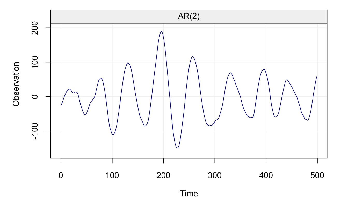
Figure 4.19: Generated AR(2) Process
fit = estimate(AR(2), Xt, demean = FALSE)
fit
## Fitted model: AR(2)
##
## Estimated parameters:
##
## Call:
## arima(x = as.numeric(Xt), order = c(p, intergrated, q), seasonal = list(order = c(P,
## seasonal_intergrated, Q), period = s), include.mean = demean, method = meth)
##
## Coefficients:
## ar1 ar2
## 1.9787 -0.9892
## s.e. 0.0053 0.0052
##
## sigma^2 estimated as 0.8419: log likelihood = -672.58, aic = 1351.15Having estimated the model’s coefficients, we can again perform the parametric bootstrap. It must be noticed that in these simulations there can be various cases where a method may fail to estimate due to numerical issues (e.g. numerically singular covariance matrices, etc.) and therefore we add a check for each estimation to ensure that we preserve those estimations that have succeeded.
B = 500
est.phi.ML = matrix(NA, B, 2)
model = AR(phi = fit$mod$coef, sigma2 = fit$mod$sigma2)

for(i in seq_len(B)) {
  set.seed(B + i)              # Set Seed for reproducibilty
  x.star = gen_gts(500, model) # Simulate the process

  # Obtain parameter estimate with protection
  # that defaults to NA if unable to estimate
  est.phi.ML[i,] = tryCatch(estimate(AR(2), x.star, demean = FALSE)$mod$coef,
  error = function(e) NA)
}
Once this is done, we can compare the bivariate distributions (asymptotic and bootsrapped) of the two estimated parameters \(\hat{\phi}_1\) and \(\hat{\phi}_2\).
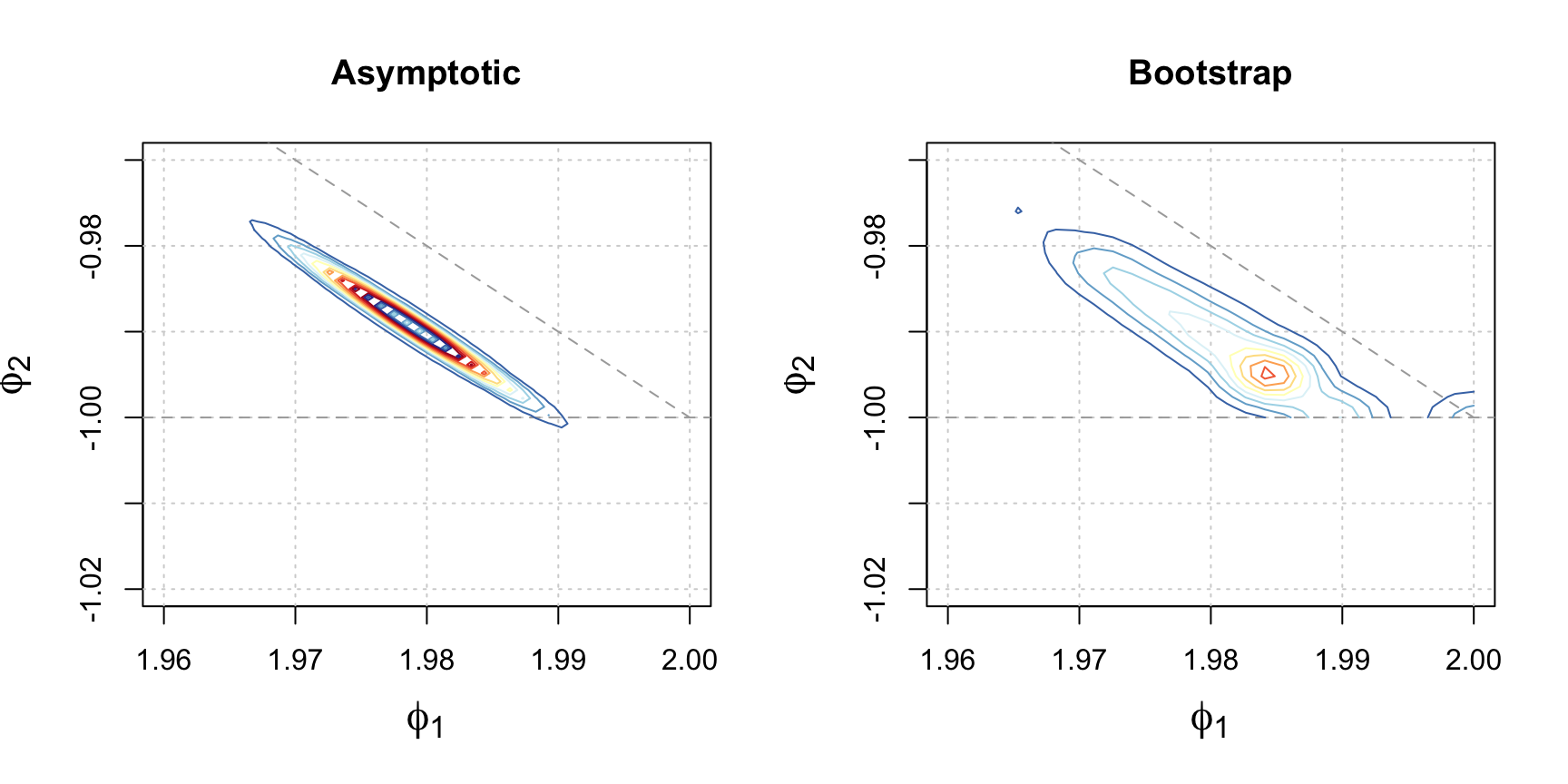
Figure 4.20: Estimated distributions of \(\hat{\phi_1}\) and \(\hat{\phi_2}\) based on the MLE using asymptotic and parametric bootstrap techniques. The colored contours represent the density of the distributions and the dark grey lines represent the boundary constraints of \(\left|\phi_2\right|<1\) and \(\phi_2 = 1 - \phi_1\).
As for any other estimation and inference procedure, these confidence intervals rely on the assumption that the chosen model (AR(2) in this case) is the true model underlying the observed time series. However, if this assumption were not correct, then the derived confidence intervals would not be correct and this could possibly lead to bad conclusions. For this reason, one could decide to use a non-parametric approach to computing these confidence intervals, such as the traditional bootstrap that consists in a simple random sampling with replacement from the original data. However, this approach would not be appropriate in the presence of dependence between observations since this procedure would break the dependence structure and therefore deliver unreliable conclusions. Therefore, to preserve the dependence structure of the original data one option would be to use block bootstrapping, which is a particular form of non-parametric bootstrap. There are many different kinds of block-bootstrap procedures for time series which are all related to the Moving Block Bootstrap (MBB) which is defined as follows.
Definition 4.4 Suppose that \(\left(X_t\right)\) is a weakly stationary time series with \(T\) observations. The procedure is as follows:
- Divide the time series into overlapping blocks \(\left\{S_1, \ldots, S_M\right\}\) of length \(\ell\), \(1 \le \ell < N\), resulting in \(M = N - \ell + 1\) blocks structured as:
\[\begin{aligned} {S_1}& = & ({X_1}, &{X_2}, \cdots , {X_\ell}) & && \\ {S_2}& = & &( {X_2}, {X_3}, \cdots , {X_{\ell + 1}}) & && \\ & \cdots & & {} & \cdots && \\ {S_M} & = & & & {} &&( {X_{N-\ell+1}}, {X_{N-\ell+2}}, \cdots , {X_{N}}) \end{aligned}\]
- Draw \(M = \left\lfloor {\frac{N}{\ell}} \right\rfloor\) blocks with replacement from these \(\left\{S_1, \ldots, S_M\right\}\) blocks and place them in order to form \((X_t^*)\).
- Compute the statistic of interest on the simulated sample \((X_t^*)\).
- Repeat Steps 2 and 3 \(B\) times where \(B\) is sufficiently “large” (typically \(100 \leq B \leq 10,000\)).
- Compute the empirical mean and variance on the statistic of interest based on the \(B\) independent replications.
The approach taken by MBB ensures that within each block the dependency between observations is preserved. However, one particular issue that now arises is that some inaccuracy is introduced as a result of successive blocks potentially being independent from each other. In reality, this is one of the trade-offs of the MBB approach that can be mitigated by selecting an optimal \(\ell\) (to improve the accuracy of the procedure one should choose \(\ell = T^{1/3}\) as \(T \to \infty\) as being the optimal choice). An earlier variant of MBB is called the Nonoverlapping Block Bootstrap (NBB) which doesn’t allow the blocks to share common data points and is presented below.
Definition 4.5 Suppose that \(\left(X_t\right)\) is weakly stationary time series with \(T\) observations.
- Divide time series into nonoverlapping blocks \(\left\{S_1, \ldots, S_M\right\}\) of length \(\ell\), \(1 \le \ell < N\), resulting in \(M = \left\lfloor {\frac{N}{\ell}} \right\rfloor\) blocks structured as:
\[\begin{aligned} {S_1}& = ({X_1}, {X_2}, \cdots , {X_\ell})& & && \\ {S_2}& = &( {X_{\ell+1}}, {X_{\ell+2}}, \cdots , {X_{2\ell}}) & && \\ & \cdots & {} & \cdots && \\ {S_K} & = & & {} &&( {X_{\left({N-\ell+1}\right)}}, {X_{N-\ell+2}}, \cdots , {X_{N}}) \end{aligned}\]
- Draw \(M\) blocks with replacement from these \(\left\{S_1, \ldots, S_M\right\}\) blocks and place them in order to form \((X_t^*)\).
- Compute the statistic of interest on the simulated sample \((X_t^*)\).
- Repeat Steps 2 and 3 \(B\) times where \(B\) is sufficiently “large” (typically \(100 \leq B \leq 10,000\)).
- Compute the empirical mean and variance on the statistic of interest based on the \(B\) independent replications.
Alternatively, depending on the case one can also use modifications of the MBB that seeks to change how the beginning and end of the time series is weighted such as a Circular Block-Bootstrap (CBB) or a Stationary Bootstrap (SB). The code below implements the MMB to obtain a bootrstrap distribution for the estimated parameters of an AR(1) model.
ar1_blockboot = function(Xt, block_len = 10, B = 500) {
  n = length(Xt)            # Length of Time Series
  res = rep(NA, B)          # Bootstrapped Statistics
  m = floor(n/block_len)    # Amount of Blocks

  for (i in seq_len(B)) {   # Begin MMB
    set.seed(i + 1199)      # Set seed for reproducibility
    x_star = rep(NA, n)     # Setup storage for new TS

    for (j in seq_len(m)) { # Simulate new time series
      index = sample(m, 1)  # Randomize block starting points
      # Place block into time series
      x_star[(block_len*(j - 1) + 1):(block_len*j)] =
      Xt[(block_len*(index - 1) + 1):(block_len*index)]
    }

  # Calculate parameters with protection
  res[i] = tryCatch(estimate(AR(1), x_star, demean = FALSE)$mod$coef,
  error = function(e) NA)
  }
  na.omit(res)              # Deliver results
}
Having defined the function above, let us consider a scenario where the model’s assumptions are not respected (i.e. wrong model and/or non-Gaussian time series). Consider an AR(1) and an AR(2) process with the same coefficients for the first lagged variable (i.e. \(\phi = \phi_1 = 0.5\)) but with different innovation noise generation procedures:
\[ \begin{aligned} \mathcal{M}_1:&{}& X_t &=0.5 X_{t-1} + W_t,&{}& W_t\sim \mathcal{N} (0,1) \\ \mathcal{M}_2:&{}& X_t &=0.5 X_{t-1} + 0.25 X_{t-2} + V_t,&{}& V_t\sim t_4 \end{aligned} \]
where \(t_4\) represents the Student-\(t\) distribution with 4 degrees of freedom (heavy tails). For the first model (\(\mathcal{M}_1\)) we will use the gen_gts() function while for the second model \(\mathcal{M}_2\) we will make use the arima.sim() function in which we can assign a vector of innovations from a \(t\) distribution.
set.seed(1)         # Set seed for reproducibilty
n = 300             # Sample size
xt_m1 = gen_gts(n, AR1(phi = 0.5, sigma2 = 1))   # Gaussian noise only
xt_m2 = gts(arima.sim(n = n, list(ar = c(0.5, 0.25), ma = 0), # Student-t noise
rand.gen = function(n, ...) rt(n, df = 4)))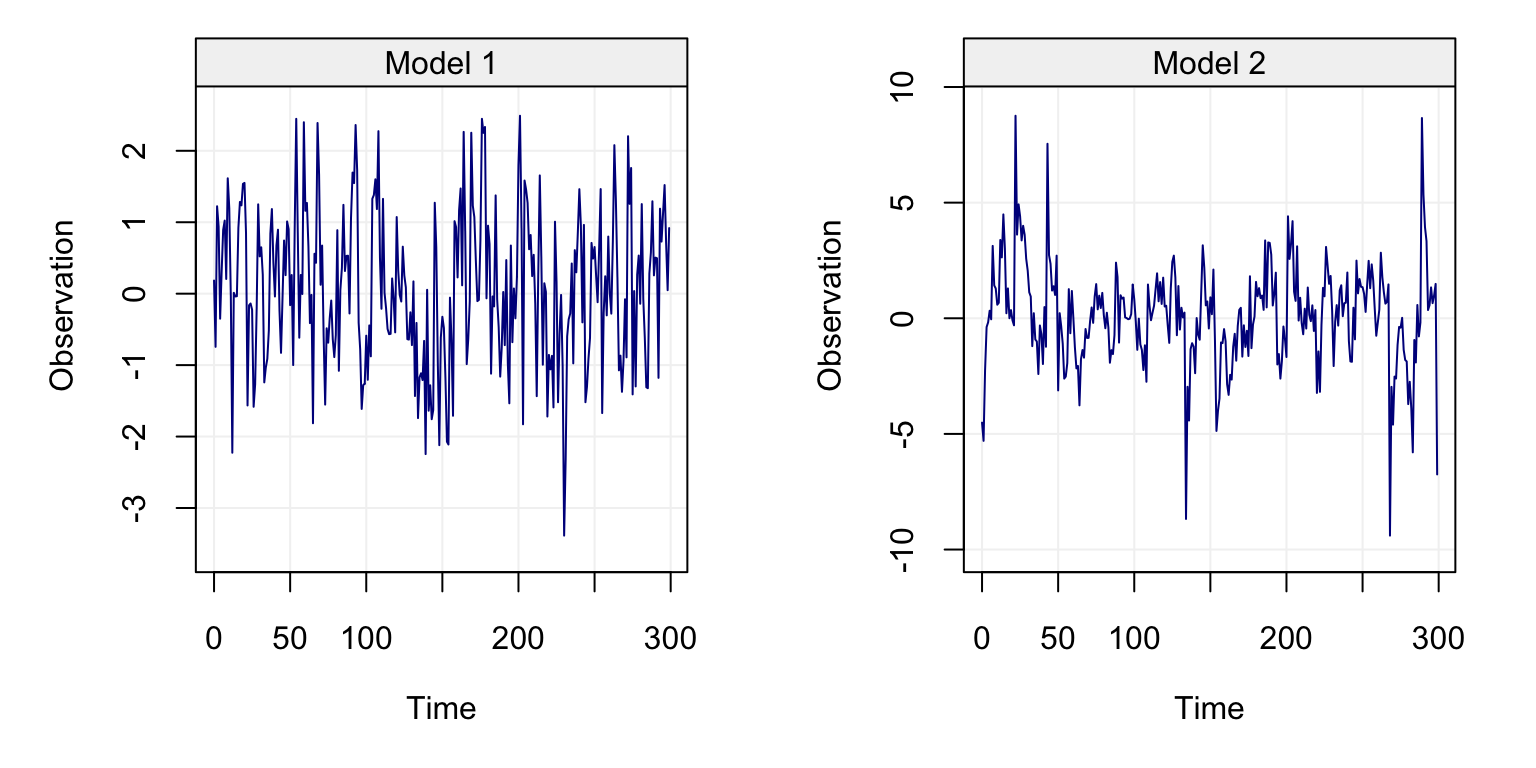
Figure 4.21: AR(1) processes generated under different noise conditions.
From Figure 4.21, the two time series appear to be considerably different as a result of the different models and noise processes. Among others, the difference is also related to the variance of the \(t\) distribution defined as \(\frac{\nu}{\nu-2}\) for \(\nu > 2\) (and \(\infty\) for \(\nu \le 2\)). Therefore, the innovation variance of the i.i.d white noise process is given by \(\sigma^2_{\mathcal{M}_1} = 1\) while the noise generated from the \(t\) distribution has innovation variance \(\sigma^2_{\mathcal{M}_2} = 2\). To compare the performance of the bootstrap procedures, the function below performs parametric bootstrap for the MLE of an AR(1) process assuming the innovations are Gaussian.
ar1_paraboot = function(model, B = 10000) {
  est.phi = rep(NA,B)    # Define a storage vector

  for(i in seq_len(B)) { # Perform bootstrap
    set.seed(B + i)      # Set seed for reproducibility
    # Simulate time series underneath the estimated model
    x.star = gen_gts(500, AR(phi = model$mod$coef, sigma2 = model$mod$sigma2))

    # Attempt to estimate parameters with recovery
    est.phi[i] = tryCatch(estimate(AR(1), x.star, demean = FALSE)$mod$coef,
    error = function(e) NA)
  }
  na.omit(est.phi)       # Return estimated phis
}
Now that we have two functions implementing the block and parametric bootstraps, we can apply these procedures to obtain confidence intervals for the (first) \(\phi\) parameter for the two time series generated respectively by model \(\mathcal{M}_1\) and \(\mathcal{M}_2\) (i.e. for \(\phi = \phi_1 = 0.5\)).
B = 1000

# Model 1
fit_m1_mle = estimate(AR(1), xt_m1, demean = FALSE)
para_m1_phi  = ar1_paraboot(fit_m1_mle, B = B)
block_m1_phi = ar1_blockboot(xt_m1, block_len = 15, B = B)

# Model 2
fit_m2_mle = estimate(AR(1), xt_m2, demean = FALSE)
para_m2_phi  = ar1_paraboot(fit_m2_mle, B = B)
block_m2_phi = ar1_blockboot(xt_m2, block_len = 15, B = B)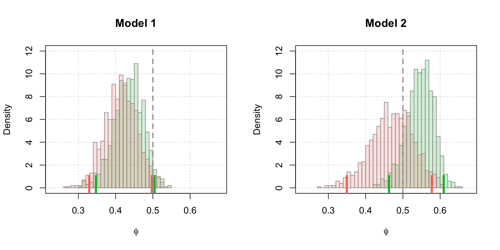
Figure 4.22: Estimated parametric and non-parametric blockbootstrap distributions of \(\hat{\phi}\) for the MLE parameter estimates. The histogram bars represent the empirical results from the bootstraps with the green representing parametric bootstrap and the red representing the block bootstrap approach. The dashed vertical line represents the true value of \(\phi\) and the vertical ticks correspond to the limits of the 95% confidence intervals for both estimation techniques.
The results from the parametric and nonparametric block bootstrapping techniques are displayed in Figure 4.22. It can be seen how, for the first model \(\mathcal{M}_1\) the parametric boostrap technique defines a confidence interval that includes the true parameter value (0.5) while the non-parametric bootstrap just misses it. In this case, being the model correctly specified for the parametric bootstrap, the latter is the preferred technique. However, it can be seen that for the second model \(\mathcal{M}_2\), the parametric bootstrap approach is greatly affected by the miss-specified model it is based on. Indeed we can see how it shifts towards larger values of \(\phi\) (although its confidence intervals still contain the true value) while the MBB remains in the proximity of the true value.
4.5 Model Selection
The diagnostic and inference tools that have been investigated this far are all based on analysing the residuals and checking the parameter confidence intervals to understand if the model is reasonable and fits the data well. However, one may be interested in understanding which, among a set of candidate models, appears to be the “best” to describe and forecast the observed time series. There are different approaches to tackling this problem among which stepwise procedures in which one starts with the simplest (or more complex) model and adds (removes) parameters until a certain statistic (criterion) is optimised. However, these approaches rely on the “paths” chosen to add the parameters (e.g. should one go from an AR(1) to an AR(2) or from an AR(1) to an MA(1)?) while there are other criteria available which are so-called “global” criteria.
The task of selecting an appropriate model is often referred to as “model selection”. In fact, this problem is a crucial part of any statistical analysis. Indeed, model selection methods become inevitable in an increasingly large number of applications involving partial theoretical knowledge and vast amounts of information, like in medicine, biology or economics. These techniques are intended to determine which variables/models are “important” to “explain” a phenomenon under investigation. The terms “important and”explain" can have very different meanings according to the context and, in fact, model selection can be applied to any situation where one tries to balance variability with complexity (McQuarrie and Tsai 1998). For example, these techniques can be applied to select “significant” variables in regression problems, to determine the order of an AR process or simply to construct histograms.
Let us consider a general criterion that we would wish a model to respect in order to be considered a “good” model. Such a criterion, that we call \(C\), could be the following:
\[\begin{equation} C = \mathbb{E}\left[ {{\mathbb{E}_0}\left[ {\left\| {{X_0} - \hat X} \right\|_2^2} \right]} \right], \tag{4.3} \end{equation}\]where \(\|X\|_2^2 \equiv X^T X\) represents the squared L2-norm, \(\hat{X}\) represents the predictions from a given (estimated) model, \(X_0\) represents future unobserved values of the time series \((X_t)\) and \(\mathbb{E}_0\) represents the out-of-sample expectation (i.e. the expectation of the future/unobserved values \(X_0\)). In general terms, this criterion is measuring the expected difference between the predicted values and the expected future/unobserved values of the time series. Therefore, a “good” model would be a model that minimizes this criterion thereby minimising the expected “prediction error” of the model. In fact, the theoretical quantity defined in (4.3) is related to Mallow’s \(C_p\) (see Mallows 1973), which is still nowadays one of the most commonly used model selection criteria for regression. Indeed, let us consider the following theorem whose proof is given in Appendix A.3.
Then, in the context of linear regression we have
\[\begin{equation*} \mathbf{Y} = \mathbf{X} \boldsymbol{\beta} + \boldsymbol{\varepsilon}, \end{equation*}\]and when considering the least-squares estimator we obtain
\[\begin{equation*} \hat{\mathbf{Y}} = \mathbf{X} \hat{\boldsymbol{\beta}} = \mathbf{X} \left(\mathbf{X}^T \mathbf{X}\right)^{-1} \mathbf{X} \mathbf{Y} = \mathbf{H} \mathbf{Y}, \end{equation*}\]where \(\mathbf{H} \equiv \mathbf{X} \left(\mathbf{X}^T \mathbf{X}\right)^{-1} \mathbf{X}\) denotes the “Hat” matrix (as it puts a 🎩 on \(\mathbf{Y}\)). Then, the theoretical \(C\) becomes:
\[\begin{equation*} C = \mathbb{E}\left[ \mathbb{E}_0 \left[ \left\| \mathbf{Y}_0 - \hat{\mathbf{Y}} \right\|_2^2 \right] \right], \end{equation*}\]and using Theorem 4.2, we obtain (why? 🤔)
\[\begin{align*} C &= \mathbb{E}\left[ \left\| \mathbf{Y} - \hat{\mathbf{Y}} \right\|_2^2 \right] + 2tr \left( \text{cov} \left( \mathbf{Y}, \hat{\mathbf{Y}} \right) \right) = \mathbb{E}\left[ \left\| \mathbf{Y} - \hat{\mathbf{Y}} \right\|_2^2 \right] + 2k \sigma^2, \end{align*}\]where \(k\) is the number of colunms of the matrix \(\mathbf{X}\) and \(\sigma^2\) the variance of the residuals \(\boldsymbol{\varepsilon}\). Thus, an unbiased estimator of \(C\) is simply
\[\begin{align*} \hat{C} &= \left\| \mathbf{Y} - \hat{\mathbf{Y}} \right\|_2^2 + 2k \sigma^2, \end{align*}\]which is known as Mallow’s \(C_p\).
Alternatively, several researchers in the 1970’s used a different approach based on the Kullback-Leibler disprepancy, which is often called the Information Theory approach. While a theoretical discussion of this method is clearly beyond the scope of this book, the general idea is essentially the same as Mallow’s \(C_p\), where one would construct a theoretical quantity (such as \(C\) in our previous example) and compute/derive a suitable estimator of this quantity. The most famous information theory-based model selection crierion is the Akaike Information Criterion or AIC (see Akaike 1974), which is probably the most commonly used model selection crierion for time series data. In the late 1970’s there was an explosion of work in this field and many model selection criteria were proposed including the Bayesian Information Criterion or BIC proposed by Schwarz and others (1978) and the HQ criterion proposed by Hannan and Quinn (1979).
All these criteria in some way represent (under different forms) the general criterion \(C\) defined earlier. Assuming that \(C\) is a good criterion to evaluate the “goodness” of a model, most of the quantites defining this criterion are not directly available and estimators are needed. Denoting \(\text{logL}(\hat{\boldsymbol{\theta}})\) as being the log-likelihood function evaluated at the estimated parameters and \(k\) as the number of parameters in the model (i.e. the length of the vector \(\boldsymbol{\theta}\)), the three criteria higlighted in the previous paragraph aim at estimating this quantity as follows:
\[\begin{align*} \text{AIC} &= -2 \text{logL}(\hat{\boldsymbol{\theta}}) + 2k\\ \text{BIC} &= -2 \text{logL}(\hat{\boldsymbol{\theta}}) + \log(T) k\\ \text{HQ} &= -2 \text{logL}(\hat{\boldsymbol{\theta}}) + 2\log(\log(T)) k . \end{align*}\]As you can notice, all three criteria have a common structure to them composed of two terms: (i) the first is a quantity that is based on the value of the likelihood function while (ii) the second is a value that depends on the number of parameters in the model \(k\) (as well as on the length of the time series \(T\)). To interpret these terms, one can consider that the first term decreases as the likelihood increases. This implies that, all other things being equal, the criterion is minimized when the value of the likelihood is the largest possible which is (always) true when the most complex model is fitted to the time series. If we were to base our choice only on this term, we would always choose the most complex model for our time series thereby leading to the problem of “overfitting” which can introduce unnecessary variability if using this model to predict future values of the time series. In order to compensate for this, the second term can be seen as a penalty-term for model complexity. Indeed, the second term increases as more parameters are added to the model.
From a theoretical standpoint it is difficult to determine which between the AIC, BIC or HQ (or many other criteria) is the best. Essentially, statisticians have considered different ways of assessing the field of model selection. The first one is known as model selection efficiency and is largely due to Shibata (1980). This paradigm relies on the common assumption (in both time series and regression) that the data generating process (or true model) is of infinite dimension and/or that the sets of candidate models (i.e. the set of models we are considering) do not include the true model. Under this setting, the goal of model selection is to find the candidate model that is the ``closest’’ to the true model. Shibata (1980) defined model selection to be asymptotically efficienct if this method chooses the candidate model with the smallest prediction error (in some sense) as the sample size goes to infinity. Under some typical conditions, the AIC as well as Mallow’s \(C_p\) are both asymptotically efficient but the BIC and HQ are not. The second approach to model selection relies on consistency and is based on the idea that the true model is of finite dimension and that it is included in the set of candidate models. Under this assumption the goal of model selection is to correctly select this true model among the candidates models. Moreover, a model selection criterion is said to be model selection consistent if it identifies the correct model with probability equal to one as the sample size goes to infinity. The BIC and HQ are both model selection consistent but this is not the case for the AIC and \(C_p\). The assumption that the true model is among the candidate models is often considered rather strong by statisticans. In practice, the efficiency approach tends to be more popular but there is little agreement and the choice between these two philosophies remains highly subjective. To make matters more confusing, both consistency and efficiency are asymptotic properties which are not “observable” in small samples. In this section, we will consider various simulations to better understand the small sample properties of AIC, BIC and HQ.
With this in mind, let us consider the use of these criteria in the selection of AR(\(p\)) models seen this far. As we saw in the previous sections, the PACF is a very useful tool to identify the order of the AR(\(p\)) model that is underlying the observed time series. However, the choice based on the PACF can possibly lead to selecting models that may adequately describe the observed time series but do not necessarily perform well in terms of prediction. For this reason, consider distinct AR(\(p\)) models with different values of \(p\):
\[\mathcal{M}_j: {X_t} = \sum\limits_{i = 1}^j {{\phi _i}{X_{t - i}}} + {W_t},\]
where \(\mathcal{M}_j\) is used to denote an AR(\(j\)) model, with \(j = 1,...,p^*\) where \(p^*\) represents the maximum order of the AR(\(p\)) model considered for a given observed time series (e.g. \(p^*\) could be the maximum lag at which the PACF appears to be significant). Let us illustrate the properties of these model selection criteria through the following example of an AR(3) model for which we show the PACF of a possible realization from this process (\(T = 500\)).
set.seed(1)
true_model = AR(phi = c(1.2, -0.9, 0.3), sigma2 = 1)
Xt = gen_gts(n = 500, model = true_model)
plot(auto_corr(Xt, pacf = TRUE))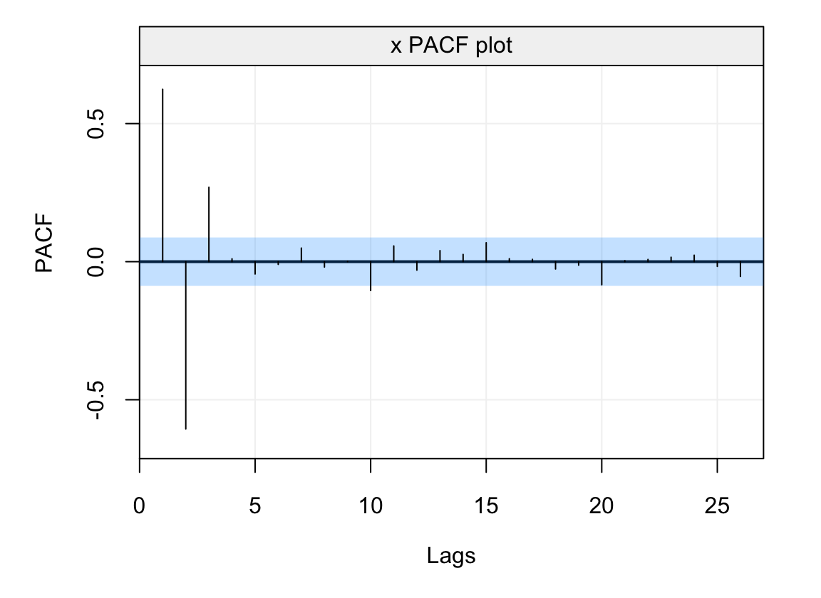
Figure 4.23: Estimated PACF of a time series from an AR(3) model with parameters \(\phi_1 = 1.2\), \(\phi_2 = -0.9\) and \(\phi_3 = 0.3\).
From the PACF plot one sees that the first three lags appear to be significant indicating that an AR(3) model would indeed appear to be a good candidate model for this observed time series. However, there is another value of the PACF that appears to be marginally significant at lag 10. Let us therefore suppose that we want to consider all possible AR(\(p\)) models with \(p^* = 10\). The select() function from the simts package allows to evaluate and plot the value of the three criteria presented earlier in order to understand the value of \(p\) that minimizes each of them.
best_model = select(AR(10), Xt, include.mean = FALSE) 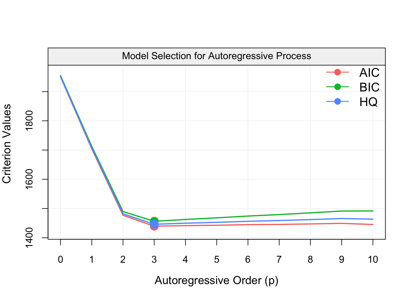
Figure 4.24: Plot of the AIC, BIC and HQ model selection criteria from all models included in an AR(10) model. The observed time series was simulated from an AR(3) model.
The output of this funtion is a plot of the values of each criterion over all possible AR(\(p\)) models with \(p = 1,...,10\) and, as can be seen from the plot, all criteria are minimized at the value \(p=3\) which shows how all criteria (in this particular case) agree and select the true underlying model. The function also delivers the MLE estimates of the parameters of the selected model:
best_model$coef## ar1 ar2 ar3
## 1.1726319 -0.8830923 0.2752257It can be seen how these estimated parameters are close to the true parameter values of the AR(3) model which was used to simulate the observed time series. Therefore the model selection criteria presented above appear to be good criteria to select the true underlying model, but they all do so in different manners. To further investigate the properties of these criteria let us consider the following simulation study.
where \(W_t \overset{iid}{\sim} \mathcal{N}(0,1).\)
The first two time series correspond to (relatively) “strong” signals (generally meaning that the values of the parameters are above 0.5) while the third is called a “weak” signal (since the parameters are mostly quite close to 0). Finally, the fourth time series is an example of an AR process of infinte dimension which corresponds to an MA(1) (which is discussed and justified further on in this chapter).
Based on the theoretical (i.e. asymptotic) properties of the considered model selection criteria, we expect the BIC to perform very well for the first two models (strong signals where the true model is among the candidate models), while the AIC should give “good” results on the last two models (weak signals with models of “larger” dimensions).
For the purpose of the simulation we consider a sample size \(T = 100\) and \(B = 1000\) bootstrap replications. The code used for the simulation study (being lengthy) is omitted for practical exposition purposes.
Figure 4.25: Barplots representing the frequency with which each considered model selection criterion (AIC, BIC, HQ) selects each of the possible candidate models within an AR(9) in each of the four simulation settings described in the text.
As anticipated, it can be seen how the BIC (green bars) often selects a small dimensional model for the first two settings, which corresponds to the truth. In these cases the AIC (red bars) performs less well compared to the other two criteria where the HQ (blue bars) appears to do better than the others for the “strong” signal AR(2). However, as the signal becomes weaker and the true model size increases (last two settings) the AIC does a better job than the BIC and the HQ since it selects higher dimensional models (which corresponds to the truth) with a higher frequency with respect to the HQ and even more so with respect to the BIC. Overall, it would appear that if a “strong” signal is present and the model dimension is low (finite), the BIC is the best choice. However, when the signal is “weaker” and the model dimension is larger (infinite), the AIC tends to select “better” models. Finally, the HQ criterion appears to be inbetween the AIC and BIC in terms of performance for the considered simulation setting.
Having studied th performance of these three criteria through the described simultation study, let us now consider an example we looked at when explaining the usefulness of the PACF to determine the order of an AR(p) model. For this reason, let us again check the PACF of the Lynx trapping data set represented below.
cor_lynx = corr_analysis(lynx_gts)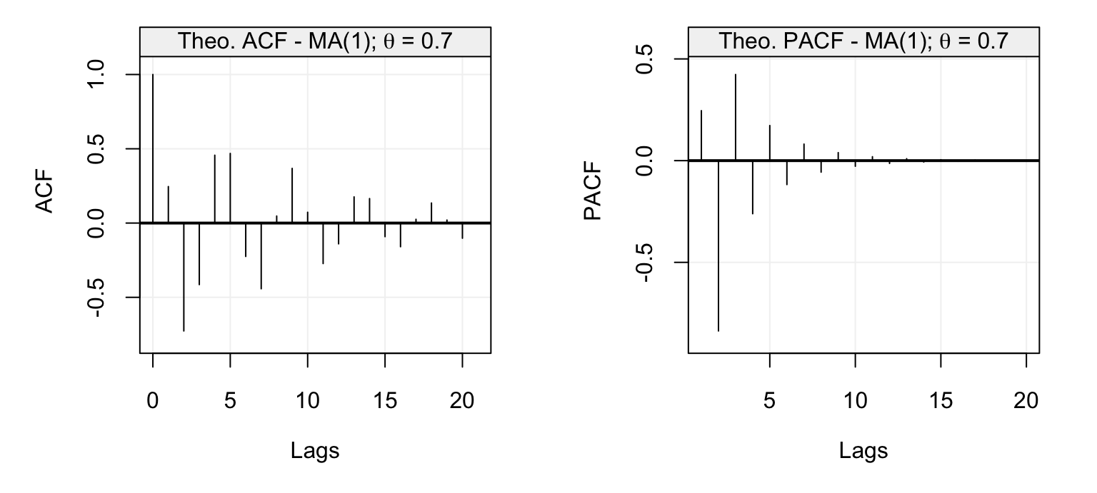
Figure 4.26: Empirical ACF and PACF of the yearly lynx trapping time series.
As we saw earlier, the PACF appears to be significant at lag \(h = 11\) therefore leading to the conclusion that an AR(11) model could be good to describe/forecast the observed time series. However, let us check if we reach the same conclusion using the three model selection criteria described above. For this reason, let us use an AR(16) as the maximum order for the candidate AR(\(p\)) models.
lynx_select = select(AR(16), lynx_gts, include.mean = TRUE)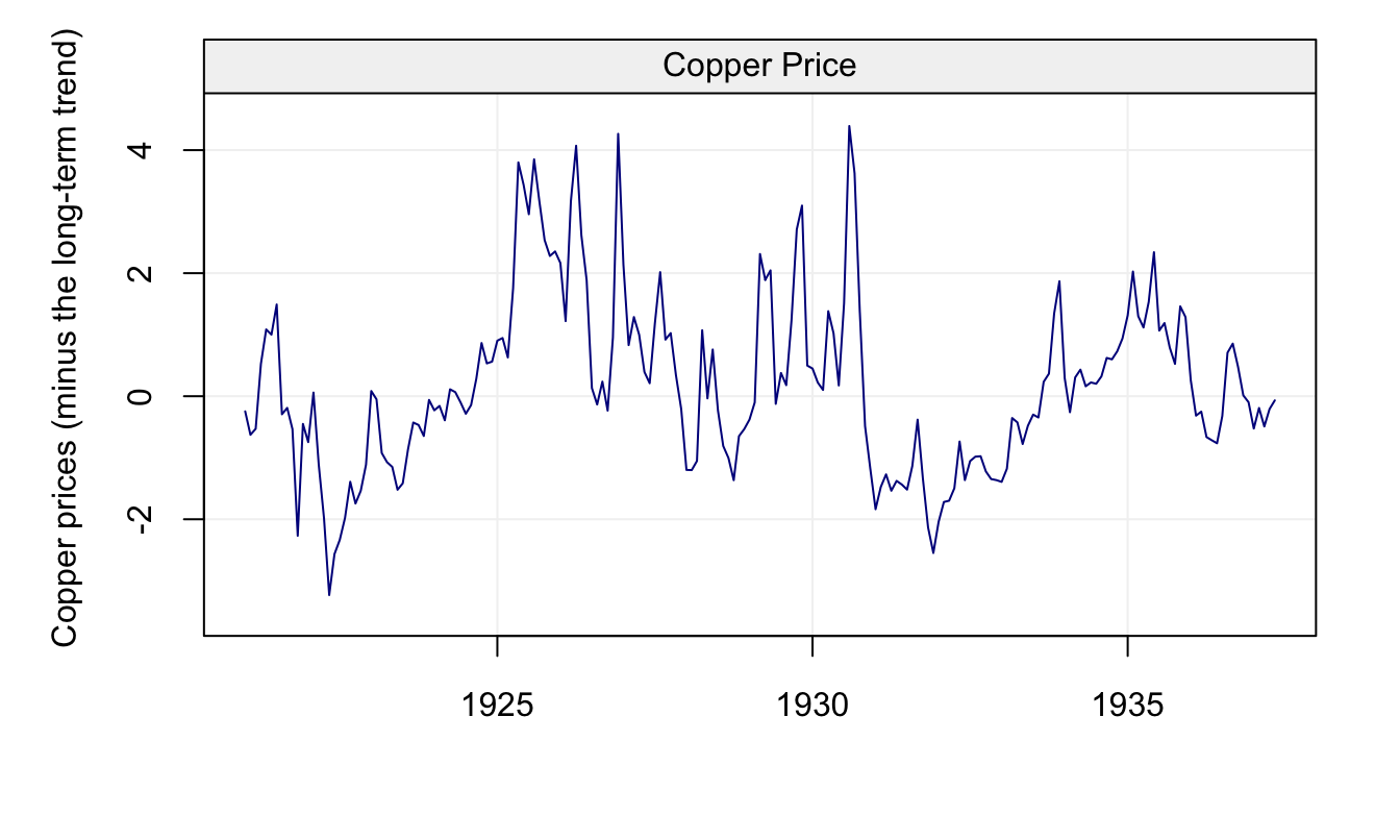
Figure 4.27: Values of the three model selection criteria described in the text for all candidate models included in an AR(16) model for the yearly lynx trapping time series.
In this case, we see that the AIC and HQ select an AR(11) model in accordance with the selection procedure based on the PACF. However the BIC selects a much smaller model (AR(2)). This is in some way consistent with the simulation study seen earlier where the BIC generally tends to select lower-dimensional models. Moreover, the true model for the lynx data may not be among the candidate models and therefore the BIC would not be a good choice. Hence, for this case the AIC or HQ are probably better choices.
To summarize, all these techniques aim at estimating the out-of-sample prediction error of a given model. However, they strongly rely on the chosen likelihood function and, if this does not adequately represent the model that generated the observed time series, then they could deliver misleading conclusions. For this reason, one could consider another approach to model-selection based on model forecasting accuracy. Indeed, one could select a model based on the following procedure:
- Split the observed time series of length \(T\) into two sub-series. The first one (i.e. training set) goes from 1 to \(n\) (where \(n\) is for example \(0.8T\)) and the second one (i.e. testing set) goes from \(n + 1\) to \(T.\)
- Estimate the model on the training set and forecast the next observation (i.e. \(X_{n+1}^n\)). Compute the difference between the forecast and the actual value \(X_{n+1}\).
- Add the observation \(X_{n+1}\) to the training set and let \(n = n + 1\). Go to Step 2 until \(n = T\).
- Compute a suitable “score” to asses the quality of the model based on the empirical “prediction errors” vector.
There are many “scores” that can assess the quality of the model using the empirical prediction errors such as the Root Mean Squared Error (RMSE), mean absolute percentage error, etc. A generally used and common score is the Median Absolute Prediction Error which is defined as follows:
\[\text{MAPE} = \text{median}\left(\Big|X_{t+j} - X_{t+j}^t\Big|\right).\]
The MAPE is a score function that assesses how far the model’s predictions are from the actual values while ensuring that a possible few outlying values cannot affect the evaluation of a model’s performance (the median is what guarantees this). This score can also be used to assess a model’s prediction performance and is implemented in the MAPE() function in the simts package (by default this function uses the first \(0.8T\) observations as training data). Let us study a few simulated examples of how the MAPE can be a “good” model selection (and evaluation) criterion. In the first example we simulate a time series from an AR(3) model and compute the MAPE on all possible candidate models within an AR(8) model.
set.seed(5)
Xt = gen_gts(500, AR(phi = c(0.1, 0, 0.8), sigma2 = 1))
MAPE(AR(8), Xt)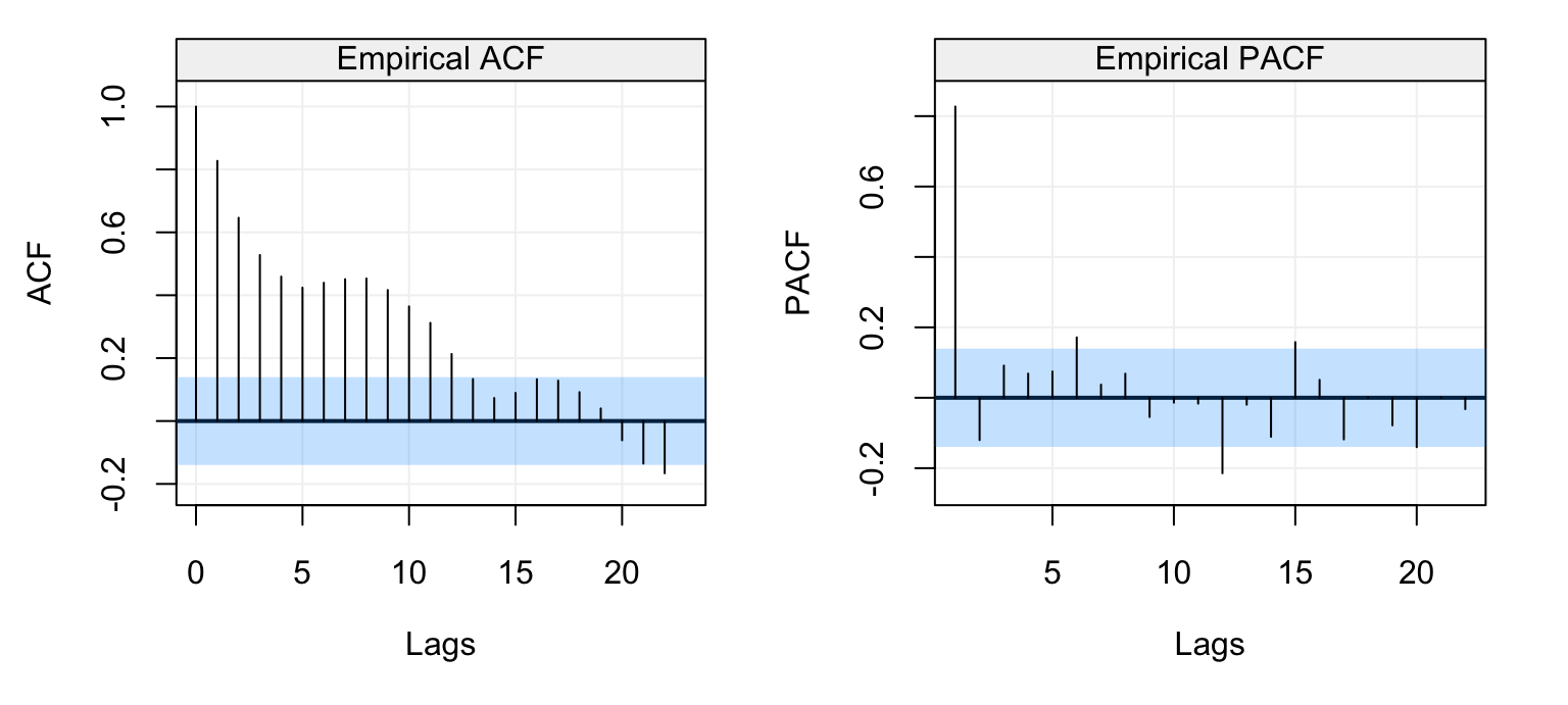
Figure 4.28: Estimated MAPE for the candidate models included in an AR(8) model. The true underlying model is an AR(3).
From the plot we can see the value of the MAPE for all models up to the AR(8) model. Aside from the MAPE itself, we can also see the confidence intervals for each value of the MAPE (representing the distance of one standard deviation from the estimated MAPE). In this example we see that the MAPE is minimized for the AR(6) (red dot) although there are other values of the MAPE that lie below the upper confidence interval of the smallest MAPE. In this case, the MAPE of the smallest model whose value lies below this bound is indeed the one corresponding to the AR(3) model and, in the optic of choosing simple models, our choice would probably fall on the latter model. Another example is simply another time series from the same model as above.
set.seed(7)
Xt = gen_gts(500, AR(phi = c(0.1, 0, 0.8), sigma2 = 1))
MAPE(AR(8), Xt)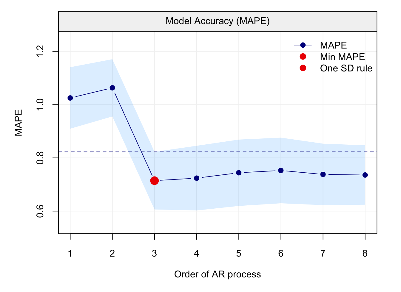
Figure 4.29: Estimated MAPE for the candidate models included in an AR(8) model. The true underlying model is an AR(3).
In this case we see that the smallest value of the MAPE corresponds to the AR(3) which is also the smallest model below the upper confidence interval of the smallest value of the MAPE (hence the green and red dots correspond, leaving only the red dot). Having studied the MAPE in a couple of examples, let us again check the lynx trappings data seen earlier when using this approach. For this purpose we use the default number of observations for the training data (i.e. the first \(0.8 \cdot T\) observations) to estimate the model and the last \(0.2 \cdot T\) to test the estimated model.
lynx_mape = MAPE(AR(16), lynx_gts)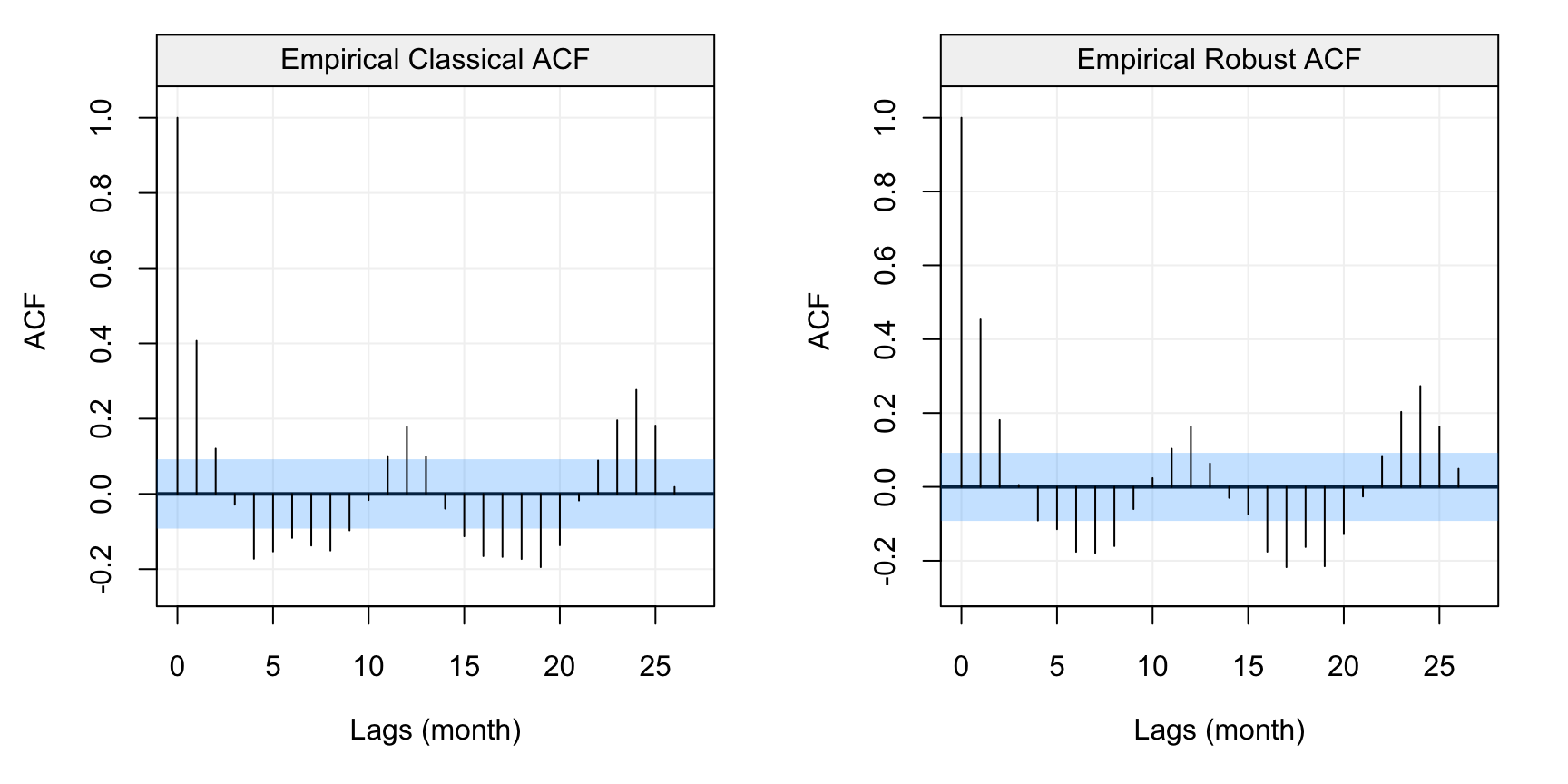
Figure 4.30: Estimated MAPE for the lynx dataset.
As we can see, an AR(11) model is selected which is equivalent to the model selected by the AIC and HQ criteria. Moveover, it can observed that MAPE is quite variable and that several models have a MAPE value close to the one of the selected model. As the MAPE is prone to overfitting, a reasonable approach is to select a model based on the “one standard deviation rule” which in this case would correspond to an AR(3), which is close to the model selected by the BIC (which is an AR(2) for this data). Therefore also this selection method would appear to indicate that either an AR(11) or an AR(2)/AR(3) appear to be “good” models for this time series.
4.6 Moving Average Models
The class of AR(\(p\)) models is a very general class that allows to take into account different forms of linear dependence between past and future observations. However, there are some forms of linear dependence that can appear as “shocks” in the innovation noise of a time series. In this sense, we have already seen a model that describes a certain form of this dependence which is the MA(1) defined as
\[X_t = \theta W_{t-1} + W_t\]
where \((W_t)\) is a white noise process. As can be seen, the observed time series \((X_t)\) is a linear combination of the innovation process. In this section we generalise this process to the class of MA(\(q\)) processes that are defined as follows.
Definition 4.6 (Moving Average of Order Q) A Moving Average of Order \(q\) or MA(\(q\)) model is defined as follows:
\[{X_t} = \theta_1 W_{t-1} + ... + \theta_q W_{t-q} + W_t,\]
where \(\theta_q \neq 0\).If we make use of the backshift operator defined earlier in this chapter, we can rewrite this model as:
\[\begin{aligned} X_t &= \theta_1 B W_t + ... + \theta_q B^q W_t + W_t \\ &= (\theta_1 B + ... + \theta_q B^q + 1) W_t .\\ \end{aligned} \]
Based on this we can deliver the following definition.
This allows us to write an MA(\(q\)) process as
\[X_t = \theta (B) W_t .\]
Following this definition, it is possible to see that an MA(\(q\)) process is always stationary. Indeed, an MA(\(q\)) respects the defintion of a linear process (see Definition 4.1) where \(\psi_0 = 1\), \(\psi_j = \theta_j\) for \(j = 1, ..., q\), and \(\psi_j = 0\) for \(j > q\) and, based on this, we can show its stationarity.
Example 4.13 (Stationarity of an MA(q) Process) Based on the above definitions, we can rewrite an MA(q) process as \(X_t = \sum\limits_{i = 0}^q {{\theta _i}{W_{t - i}}}\), where \(\theta_0 = 1\) and assume the condition that \(\sum\limits_{j = 0}^q {\theta _j^2} < \infty\) (if \(\theta_j < \infty\) for all \(j\) and \(q < \infty\), this condition is verified). Using this expression we start verifying (weak) stationarity by checking the expectation of an MA(q) process which is given by
\[\mathbb{E}\left[ X_t \right] = \mathbb{E}\left[ \sum\limits_{i = 0}^q {{\theta _i}{W_{t - i}}} \right] = \sum\limits_{i = 0}^q {{\theta _i}} \mathbb{E}\left[ {W_{t - i}} \right] = 0,\]
which confirms that the expectation is constant. We now have to verify the conditions on the autocovariance function which is derived as follows:
\[\begin{align} \text{cov}\left( {{X_{t + h}},{X_t}} \right) &= \text{cov} \left( {\sum\limits_{j = 0}^q {{\theta _j}{W_{t + h - j}}} ,\sum\limits_{i = 0}^q {{\theta _i}{W_{t - i}}} } \right) \\ &= \sum\limits_{j = 0}^q {\sum\limits_{i = 0}^q {{\theta _j}{\theta _i} \;\text{cov} \left( {{W_{t + h - j}},{W_{t - i}}} \right)} } \\ &= \sum\limits_{j = 0}^q {\sum\limits_{i = 0}^q {{\theta _j}{\theta _i}\; \underbrace {\text{cov} \left( {{W_{t + h - j}},{W_{t - i}}} \right)}_{ = 0 \, \text{for} \, i \neq j - h}} } + {1_{\left\{ {\left| h \right| \leqslant q} \right\}}}\sum\limits_{j = 0}^{q - \left| h \right|} {{\theta _{j + \left| h \right|}}{\theta _j} \;\underbrace{\text{cov} \left( {{W_t},{W_t}} \right)}_{= \sigma^2}} \\ &= {1_{\left\{ {\left| h \right| \leqslant q} \right\}}}{\sigma ^2}\sum\limits_{j = 0}^{q - \left| h \right|} {{\theta _{j + \left| h \right|}}{\theta _j}} \end{align}\]As a result, we have:
\[{1_{\left\{ {\left| h \right| \leqslant q} \right\}}}{\sigma ^2}\sum\limits_{j = 0}^{q - \left| h \right|} {{\theta _{j + \left| h \right|}}{\theta _j}} \leqslant {\sigma ^2}\sum\limits_{j = 0}^q {\theta _j^2} < \infty. \]
Given these results, we also have
\[\text{var}(X_t) = {\sigma ^2}\sum\limits_{j = 0}^q {\theta _j^2},\]
which (under our assumption) is finite and does not depend on time. Moreover, the covariance only depends on the lag \(h\) (not on the time \(t\)) and, therefore, an MA(\(q\)) process is weakly stationary.
Although an MA(\(q\)) process is always weakly stationary, it is important to well define these models since they can be characterized by certain parametrizations that don’t allow them to be uniquely identified. Indeed, the latter issues can be fall within the problem of model identifiability in which different MA(\(q\)) models (of the same order \(q\)) can produce identical autocovariance functions.
Example 4.14 (Non-uniqueness of MA models) For example, consider the following two MA(1) processes:
\[ \begin{aligned} X_t &= \frac{1}{\theta}W_{t-1} + W_t,&{}& W_t \overset{iid}{\sim} \mathcal{N} (0, \sigma^2\theta^2), \\ Y_t &= \theta Z_{t-1} + Z_t,&{}& Z_t \overset{iid}{\sim} \mathcal{N} (0,\sigma^2). \end{aligned} \]
By observation, one can note that the models share the same expectation:
\[\mathbb{E}\left[ {{X_t}} \right] = \mathbb{E}\left[ {{Y_t}} \right] = 0.\]
As for the autocovariance, this is derived in the following manner
\[\begin{align} \text{cov} \left( {{X_t},{X_{t + h}}} \right) &= \text{cov} \left( {{W_t} + \frac{1}{\theta }{W_{t - 1}},{W_{t + h}} + \frac{1}{\theta }{W_{t + h - 1}}} \right)\\ &= {\boldsymbol{1}_{\left\{ {h = 0} \right\}}}{\sigma^2}(1 + {\theta ^2}) + {\boldsymbol{1}_{\left\{ {\left| h \right| = 1} \right\}}}\frac{{{\sigma ^2}{\theta ^2}}}{\theta }\\ &= {\sigma ^2}\left( {{\boldsymbol{1}_{\left\{ {h = 0} \right\}}}(1 + {\theta^2}) + {\boldsymbol{1}_{\left\{ {\left| h \right| = 1} \right\}}}\theta } \right) \\[12pt] \text{cov} \left( {{Y_t},{Y_{t + h}}} \right) &= \text{cov} \left( {{Z_t} + \theta {Z_{t - 1}},{Z_{t + h}} + \theta {Z_{t + h - 1}}} \right)\\ &= {\boldsymbol{1}_{\left\{ {h = 0} \right\}}}{\sigma ^2}(1 + {\theta ^2}) + {\boldsymbol{1}_{\left\{ {\left| h \right| = 1} \right\}}}{\sigma ^2}\theta\\ &= {\sigma ^2}\left( {{\boldsymbol{1}_{\left\{ {h = 0} \right\}}}(1 + {\theta ^2}) + {1_{\left\{ {\left| h \right| = 1} \right\}}}\theta } \right). \end{align}\]From this we can see that \(\text{cov} \left( {{X_t},{X_{t + h}}} \right) = \text{cov} \left( {{Y_t},{Y_{t + h}}} \right)\), for all \(h \in \mathbb{Z}\). Using this result and since the innovations of the two processes are Gaussian we have:
\[\mathbf{X}_T \sim \mathcal{N} \left(\mathbf{0}, \boldsymbol{\Sigma}\right), \;\;\; \text{and} \;\;\; \mathbf{Y}_T \sim \mathcal{N} \left(\mathbf{0}, \boldsymbol{\Sigma}\right)\]
where \[\mathbf{X}_T \equiv \left[ {\begin{array}{*{20}{c}} {{X_1}} \\ \vdots \\ {{X_T}} \end{array}} \right],\mathbf{Y}_T \equiv \left[ {\begin{array}{*{20}{c}} {{Y_1}} \\ \vdots \\ {{Y_T}} \end{array}} \right],\]
and where
\[\boldsymbol{\Sigma} \equiv {\sigma ^2}\left[ {\begin{array}{*{20}{c}} {\left( {1 + {\theta ^2}} \right)}&\theta &0& \cdots &0 \\ \theta &{\left( {1 + {\theta ^2}} \right)}&\theta &{}& \vdots \\ 0&\theta &{\left( {1 + {\theta ^2}} \right)}&{}&{} \\ \vdots &{}&{}& \ddots &{} \\ 0& \cdots &{}&{}&{\left( {1 + {\theta ^2}} \right)} \end{array}} \right].\]
Therefore the two process are completely indistinguishable as they have the same distribution (as highlighted in Chapter 2). In Statistics, they are said to be non-identifiable.
Naturally, the identifiability issues discussed in Example 4.14 are of considerable importance to tackle especially when attempting to estimate the parameters of an MA(\(q\)) model. For the purpose of illustration, let us again consider the same setting with an MA(1) process in the example below.
Example 4.15 (Non-injectivity of the Likelihood function for MA models) Using the same setting as in Example 4.14, we will verify that likelihood is not injective (which is rather trivial). Indeed, \(\mathbf{X}_T\) follows a multivariate normal distrbution with mean \(\mathbf{0}\) and covariance matrix \(\boldsymbol{\Sigma}\) and therefore likelihood function for an MA(1) is the following:
\[L\left( {\boldsymbol{\beta} |\mathbf{X}_T} \right) = {\left( {2\pi } \right)^{ - \frac{T}{2}}}{\left| \boldsymbol{\Sigma}(\boldsymbol{\beta}) \right|^{ - \frac{1}{2}}}\exp \left( { - \frac{1}{2}{\mathbf{X}_T^T}{\boldsymbol{\Sigma}(\boldsymbol{\beta})^{ - 1}}\mathbf{X}_T} \right),\]
where \(\boldsymbol{\beta} \equiv [\theta \;\;\; \sigma^2]^T\). Then, it is easy to see that if we take
\[{\boldsymbol{\beta}_1} = \left[ {\begin{array}{*{20}{c}} \theta \\ {{\sigma ^2}} \end{array}} \right]\;\;\; \text{and}\;\;\;{\boldsymbol{\beta}_2} = \left[ {\begin{array}{*{20}{c}} {\frac{1}{\theta }} \\ {{\sigma ^2}\theta } \end{array}} \right],\]
we will have
\[L\left( {\boldsymbol{\beta}_1} |\mathbf{X}_T \right)= L\left( {\boldsymbol{\beta}_2} |\mathbf{X}_T \right),\]
since \(\boldsymbol{\Sigma}(\boldsymbol{\beta}_1)=\boldsymbol{\Sigma}(\boldsymbol{\beta}_2)\). This non-injectivity of the likelihood is problematic since the MLE is the value of \(\boldsymbol{\beta}\) that maximzes the likelihood function. Therefore, in this case the solution will not be unique.
Given the identifiability issues illustrated in Examples 4.14 and 4.15, the accepted rule to choose which MA(\(q\)) model to estimate (among equivalent order models) is to only consider the MA(\(q\)) models that, when rewritten in an AR(\(p\)) form, can be defined as being AR(\(\infty\)) models. These models are called invertible.
Example 4.16 (Invertibility of MA(1) models) Let us consider an MA(1) model
\[X_t = \theta W_{t-1} + W_t,\]
which can be rewritten as
\[W_t = -\theta W_{t-1} + X_t.\]
Now, the MA(1) model has taken the form of an AR(1) model and, using the recursive approach that we used to study the AR(\(p\)) models, we can show that we get to the form
\[W_t = (-\theta)^t W_0 + \sum_{j = 0}^t (-\theta)^j X_{t-j}.\]
If we assume \(|\theta| < 1\), then we finally get to the causal AR(\(p\)) representation
\[W_t = \sum_{j = 0}^{\infty} (-\theta)^j X_{t-j}.\]Therefore, between two MA(1) models with two identical ACFs, we choose the invertible MA(1) which respects the condition \(|\theta| < 1\). The same reasoning as for causal AR(\(p\)) models is also applied for invertible MA(\(q\)) models thereby restricting the possible values of the parameters of an MA(\(q\)) model to the admissable region defined in the same way as for causal AR(\(p\)) models. This reasoning also allows us to study MA(\(q\)) models similarly to AR(\(p\)) models as follows.
Definition 4.8 (Invertible MA models) If an MA(q) model can be written as follows
\[\theta^{-1}(B) X_t = W_t,\]
where \(\theta(B)\) is the moving average operator then the MA(q) model is invertible.4.6.1 The Autocovariance Function of MA processes
In this section, we will briefly discuss the behaviour of the ACF and PACF of MA(\(q\)). As an example let us consider the following four MA(\(q\)) models:
\[ \begin{aligned} Q_t &= 0.9 W_{t-1} + W_t \\ X_t &= -0.9 W_{t-1} + W_t \\ Y_t &= 1.2W_{t-1} -0.3 W_{t-2}+ W_t \\ Z_t &= -1.5 W_{t-1} + 0.5 W_{t-2} - 0.2 W_{t-3} + W_t. \end{aligned} \]
The theoretical ACF plots of these four models are shown below.
par(mfrow = c(2,2))
plot(theo_acf(ar = 0, ma = 0.9))
plot(theo_acf(ar = 0, ma = -0.9))
plot(theo_acf(ar = 0, ma = c(1.2, -0.3)))
plot(theo_acf(ar = 0, ma = c(-1.5, 0.5, -0.2)))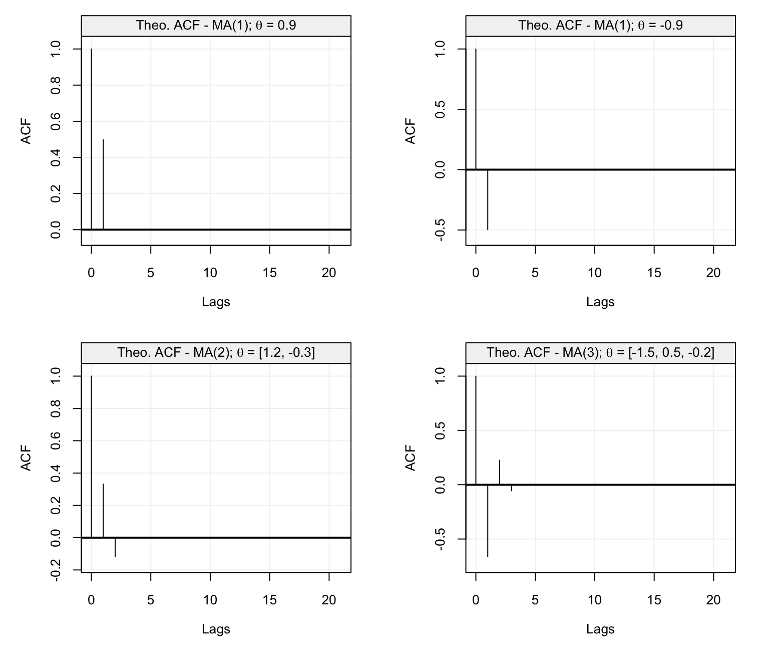
Figure 4.31: Theoretical ACF of four MA models with parameters defined in the text.
As you can notice, the values of the ACF plots become zero as soon as the lag of the ACF goes beyond the order \(q\) of the MA(\(q\)) model. Hence, the ACF plot of an MA(\(q\)) model plays the same role that the PACF plays for AR(\(p\)) models: it helps determine the order \(q\) of the MA(\(q\)) process generating a given time series. Let us now consider the PACF plots of the same models defined above.
par(mfrow = c(2,2))
plot(theo_pacf(ar = 0, ma = 0.9))
plot(theo_pacf(ar = 0, ma = -0.9))
plot(theo_pacf(ar = 0, ma = c(1.2, -0.3)))
plot(theo_pacf(ar = 0, ma = c(-1.5, 0.5, -0.2)))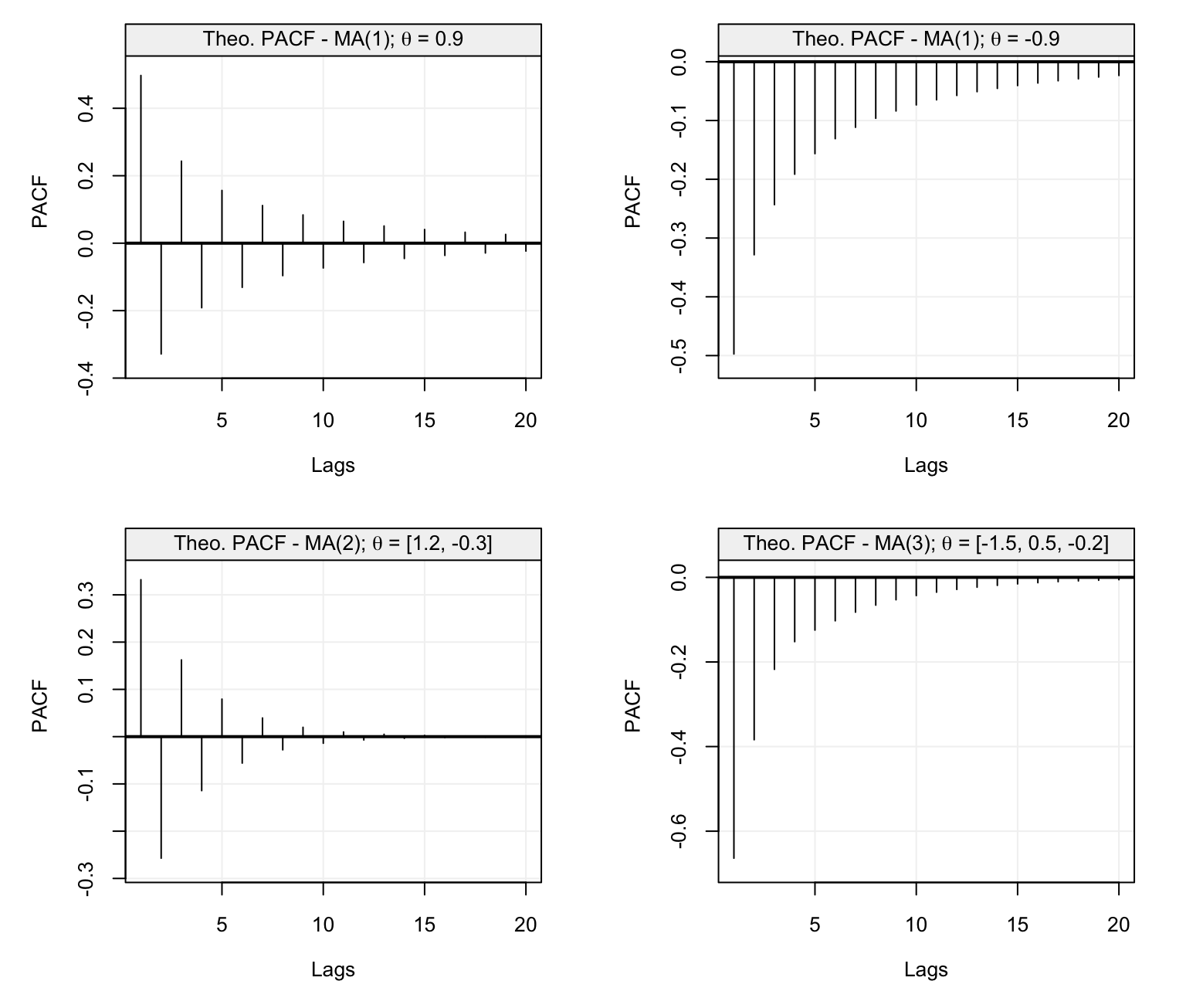
Figure 4.32: Theoretical PACF of four MA models with parameters defined in the text.
In this case, we can see that the PACF plots show a certain exponential (sinusoidal) decay that is usually observed in the ACF plots of AR(\(p\)) models. Therefore, the roles of the ACF and PACF in identifying the kind of AR(\(p\)) models underlying an observed time series is completely inversed when considering MA(\(q\)) models. Indeed, the PACF plot of an MA(\(q\)) model has an exponential decay while the ACF cuts off after the lag has reached the order of the model (\(q\) for MA(\(q\)) models).
To understand how this information can be useful when studying time series, let us simulate \(T = 200\) observations from \((X_t)\) to obtain the following time series:
set.seed(6)
Xt = gen_gts(MA(theta = 0.9, sigma2 = 1), n = 200)
plot(Xt)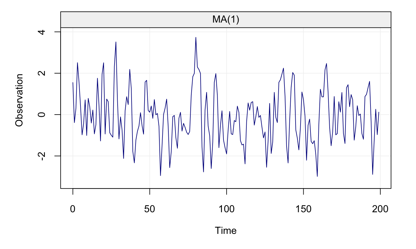
Figure 4.33: Simulated MA(1) Process
Using this data, let us estimate the ACF and PACF of this time series.
corr_ma1 = corr_analysis(Xt)
Figure 4.34: Empirical ACF and PACF of the previously simulated MA(1).
From these plots, using the PACF we could conclude that this function appears to decay as the lags increase (as the PACF of an MA(\(q\)) model is expected to do) while using the ACF we could state that the correct order for the MA(\(q\)) model is \(q = 1\) since the ACF does not appear to be significant after lag 1.
4.6.2 Selecting and Forecasting MA(\(q\)) Models
Let us now also consider the model selection criteria described in the previous section by applying the select() function to the previously simulated time series from an MA(1) model.
select_ma = select(MA(10), Xt, include.mean = FALSE)
Figure 4.35: Values of the three model selection criteria for all candidate models included in an MA(10) model for the previously simulated MA(1).
As for the conclusion based on the ACF, also in this case we see that the model selection criteria all tend to agree with each other on the fact that the best model to describe the observed time series is indeed an MA(1) model. For the purpose of illustration, let us again consider the Lynx data seen in the model selection section. From the ACF and PACF plot the choice of an AR(\(p\)) model appears to be more reasonable compared to that of an MA(\(q\)) model. Let us nevertheless understand how well an MA(\(q\)) model can fit the observed time series and, for this reason, let us perform a model selection procedure to choose the order \(q\) for the MA(\(q\)) model within the set of possible models within an MA(16).
select_lynx = select(MA(16), lynx_gts)
Figure 4.36: Values of the three model selection criteria for all candidate models included in an MA(16) model for the yearly Lynx trappings.
In this case all criteria appear to agree on the value \(q = 10\). Given that the best model for the class of AR(\(p\)) models was an AR(11), let us compare these two models when estimating them on the lynx time series.

Figure 4.37: Diagnostic plots for the residuals of a fitted AR(11) model on the yearly Lynx trappings.

Figure 4.38: Diagnostic plots for the residuals of a fitted MA(10) model on the yearly Lynx trappings.
From the diagnostic plots we can observe that both models appear to be doing a realtively good job (although the AR(11) appears to be better) so they could both be considered candidates to describe and forecast the values of the Lynx trappings. However, let us use a model selection criterion to compare them (e.g. AIC).
AIC(lynx_ar)## [1] 166.1338AIC(lynx_ma)## [1] 181.5452Therefore, based on the AIC, we would nevertheless choose to model this time series using an AR(11) model. Supposing however that we had chosen the MA(10) model to describe and predict our time series: how would we deliver forecasts based on this model?
Example 4.17 (Forecasting MA models) Let us assume we want to deliver a one-step ahead forecast based on an MA(\(q\)) model. This is given by the conditional expectation
\[X_{t+1}^t = \mathbb{E}\left[X_{t+1} | X_t, ..., X_1, W_t ..., W_1\right] = \theta_1 W_t + ... + \theta_q W_{t-q+1}.\]
However, we do not observe the innovation process \((W_t)\) directly and therefore forecasting MA(\(q\)) models is more complicated than forecasting AR(\(p\)) models. For this reason there are different techniques such as the innovation algorithm or the Kalman filter that allow to deliver these forecasts. These techniques however are out of the scope of this book.4.7 Autoregressive Moving Average Models ⚠️
The classes of time series models discussed this far (i.e. AR(\(p\)) and MA(\(q\)) models) are both classes that address different forms of dependence between observations over time. The class of AR(\(p\)) models describes the direct (and indirect) linear dependence between observations over time while MA(\(q\)) models describe the dependence in the innovation processes rather than the observations themselves. Separately, these classes of models therefore allow to take into account two extremely common dependence settings within time series. In this section however we present a class of models that combines the features of these two classes and are called ARMA(\(p\),\(q\)) models. These are defined as follows.
Based on this definition, we can see how ARMA(\(p\),\(q\)) models allow to take into account the two forms of dependence of the previous classes of models and generalize them. Indeed, if we fix \(q = 0\), an ARMA(\(p\),\(q\)) model simply becomes an AR(\(p\)) model while, on the contrary, if we fix \(p = 0\) these models become MA(\(q\)) models. Hence, the class of ARMA(\(p\),\(q\)) models is an extremely flexible class which inherits the properties (and constraints) of the two classes of models discussed this far.
Given these conditions, we can now define the conditions for the ARMA(\(p\),\(q\)) models we are going to consider in this section.
Definition 4.10 (Causal and Invertible ARMA(p,q) models) An ARMA model is causal and invertible if:
- the AR(\(p\)) part is causal, and
- the MA(\(q\)) part is invertible
If the above conditions are respected, then we are sure to be working with ARMA models that are stationary and whose parameters can be uniquely identified. This is a direct consequence of the separate properties and conditions for AR(\(p\)) models, on one side, and MA(\(q\)) models, on the other side. However, there are additional “constraints” that need to be considered given the wider class of dependence that ARMA models can take into account. Indeed, with the copresence of AR(\(p\)) and MA(\(q\)) models can lead to the definition of ARMA(\(p\),\(q\)) models that can be re-expressed as another ARMA(\(p*\),\(q*\)) model where \(p \leq p*\) and/or \(q \leq q*\). Remember that the identifiability issue for MA(\(q\)) models exists only for models with the same order \(q\) so this is a different setting. This issue for ARMA models is called “parameter redundancy”.
Based on the expression above, we can see that both sides of the ARMA equation share a common term which is \((1 - 0.9B)\) which therefore can be simplified thereby defining the mode \[X_t = W_t.\]
Hence, the specified ARMA(1,1) model is actually a white noise mode.In general, if a model has autoregressive and moving average operators that share a common root, then the model has redundant parameters and can consistute an “over-parametrization” of the problem. Let us further explore this problem through another example.
As a result of this, it is important to define (and estimate) ARMA models that are not an over-parametrization of a more “simple” ARMA model.
4.7.1 Autocovariance of ARMA Models
Since ARMA(\(p\),\(q\)) models are a class of models that inherits much of the properties of AR(\(p\)) and MA(\(q\)) models, as for their properties in terms of stationarity and identifiability, they also inherit much of the characteristics of the previously defined models in terms of their autocovariance (autocorrelation) functions. However, while the analytical derivation of the autocovariance functions for AR(\(p\)) and MA(\(q\)) models was a relatively feasible task, this is less the case for ARMA models.
Example 4.21 (Autocorrelation of an ARMA(1,1)) For an ARMA(1,1) we have
\[\rho(h) = \phi^{h-1} \rho(1)\]
where
\[\begin{equation*} \rho(1) = \frac{\left(1+\theta \phi \right)\left(\theta + \phi\right)}{1+2\phi\theta+\theta^2}. \end{equation*}\]From the above example we can observe how for the lowest order ARMA model the autocorrelation function assumes a much more complex structure compared to those presented in the previous sections for AR(\(p\)) and MA(\(q\)) models. This is even more the case for higher order ARMA models and, for this reason, aside from brute-force calculation of the ACF for specific ARMA models, different software make these computations based on user-provided parameter values.
Aside from the actual derivation of the ACF (and PACF) of ARMA models, another aspect of these models that cannot be directly transferred from the AR(\(p\)) and MA(\(q\)) models described earlier is the ease of interpretation of their ACF and PACF plots. Indeed, as we saw in the previous sections, the ACF and PACF plots of AR(\(p\)) and MA(\(q\)) models are quite informative in terms of understanding which of the two classes of models an observed time series could have been generated from and, once this has been decided, which order (\(p\) or \(q\)) is the most appropriate. However, this is not the case anymore for ARMA(\(p\),\(q\)) models since they’re a result of the combination of the two previous classes and it’s (almost) impossible to distinguish which features of the ACF and PACF belong to which part of the ARMA(\(p\),\(q\)) model.
The table below summarizes the characteristics of the ACF and PACF plots for the three classes of models discussed this far.
| AR(\(p\)) | MA(\(q\)) | ARMA(\(p\),\(q\)) | |
|---|---|---|---|
| ACF | Tails off | Cuts off after lag \(q\) | Tails off |
| PACF | Cuts off after lag \(p\) | Tails off | Tails off |
As highlighted in the table, the first two classes have distinctive features to them while the class of ARMA(\(p\),\(q\)) models have similar characteristics for both ACF and PACF plots. To better illustrate these concepts, let us consider the following two ARMA(\(p\),\(q\)) models:
\[ \begin{aligned} X_t &= 0.3 X_{t-1} - 0.8 X_{t-2} + 0.7 W_{t-1} + W_t \\ Y_t &= 1.2 X_{t-1} - 0.25 X_{t-2} - 0.1 W_{t-1} - 0.75 W_{t-2} + W_t, \\ \end{aligned} \]
where \(W_t \overset{iid}{\sim} \mathcal{N}(0, 1)\). The first model is an ARMA(2,1) model while the second is an ARMA(2,2) model and, as can be seen, the parameters between these two models are quite different. The figures below show a realization from each of these two models for time series of length \(T=500\).
Xt = gen_gts(n = 500, ARMA(ar = c(0.3,-0.8), ma = 0.7, sigma2 = 1))
Yt = gen_gts(n = 500, ARMA(ar = c(1.2, -0.25),
             ma = c(-0.1, -0.75), sigma2 = 1))
par(mfrow = c(2,1))
plot(Xt, main = expression("Simulated process: "* X[t] *" with "* T *" = 500"))
plot(Yt, main = expression("Simulated process: "* Y[t] *" with "* T *" = 500"))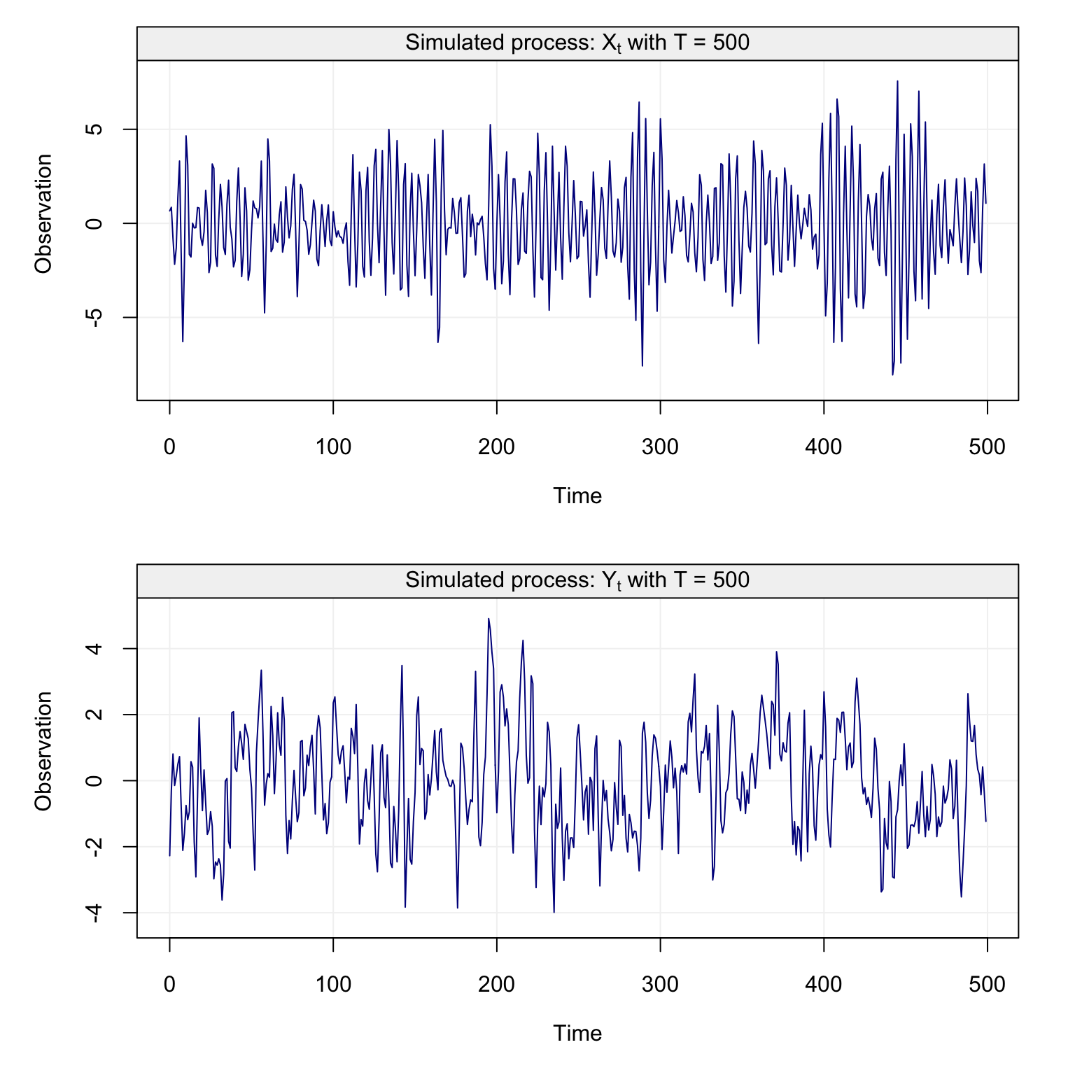
Figure 4.39: Plots of simulated time series from an ARMA(2,1) model (top plot) and from an ARMA(2,2) model (bottom plot)
As for the previous classes of models, a direct plot of the time series doesn’t necessarily allow to acquire much information on the possible models underlying the data. Let us consequently consider the theoretical ACF and PACF plots of these two models to understand if we can obtain more information.
par(mfrow = c(1,2))
plot(theo_acf(ar = c(0.3,-0.8), ma = 0.7), main = expression("Theo. ACF - MA(1); "* theta *" = 0.7"))
plot(theo_pacf(ar = c(0.3,-0.8), ma = 0.7), main = expression("Theo. PACF - MA(1); "* theta *" = 0.7"))
Figure 4.40: Theoretical ACF (left plot) and PACF (right plot) for the ARMA(2,1) model defined in the text.
par(mfrow = c(1,2))
plot(theo_acf(ar = c(1.2, -0.25), ma = c(-0.1, -0.75)), main = expression("Theo. ACF - MA(2); "* theta *" = -0.75"))
plot(theo_pacf(ar = c(1.2, -0.25), ma = c(-0.1, -0.75)), main = expression("Theo. PACF - MA(2); "* theta *" = -0.75"))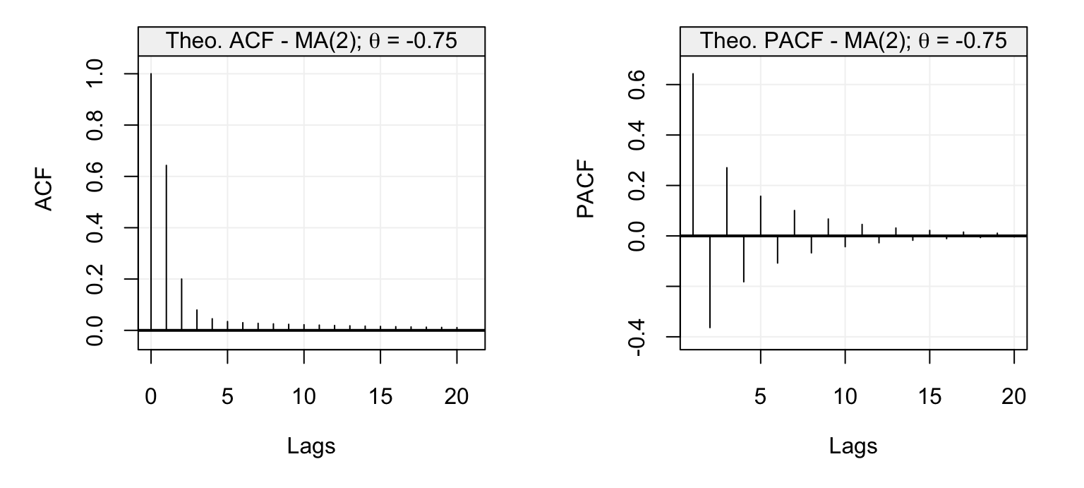
Figure 4.41: Theoretical ACF (left plot) and PACF (right plot) for the ARMA(2,2) model defined in the text.
As can be seen from the ACF and PACF plots of these two models, it would be complicated to determine what type of model and what order would be more appropriate. For this reason, for ARMA(\(p\),\(q\)) models the ACF and PACF plots can only help to understand if the autocovariance has a reasonable behaviour (e.g. tails off as the lags increase) or, for example, if there appears to be some deterministic trends and/or seasonalities are left in the data. Therefore, a more reasonable (and simple) approach to understand if an ARMA(\(p\),\(q\)) is appropriate is via a model selection criterion or an estimator of the out-of-sample predicition error (e.g. MAPE). Once this is done, the selected model(s) can fit to the observed time series and a residual analysis can be performed in order to understand if the chosen model(s) appear to do a reasonable job.
Let us illustrate the above procedure through another applied example. The time series shown in the figure below represents the annual copper prices from 1800 to 1997 (with the long-term trend removed) which can be downloaded in R via the tsdl library.
copper_ts = as.numeric(subset(tsdl, description = "copper")[[3]])
time = 1:length(copper_ts)
detrend_copper_ts = lm(copper_ts ~ time)$residuals
Xt = gts(detrend_copper_ts,
    start = 1800, freq = 1, name_ts = "Copper prices (minus the long-term trend)",
    data_name = "Copper Price", name_time = "")
plot(Xt)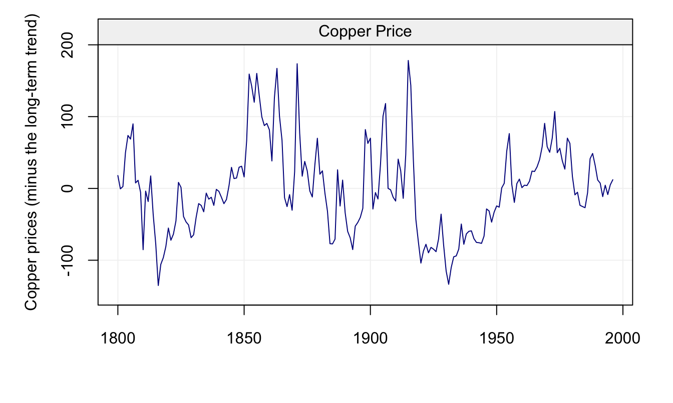
Figure 4.42: Annual Prices of Copper from 1880-1997 with long-term trend removed.
It would appear that the process could be considered as being stationary and, given this, let us analyse the estimated ACF and PACF plots for the considered time series.
corr_analysis(Xt)
Figure 4.43: Empirical ACF (left) and PACF (right) of the annual copper prices.
The ACF plot could eventually suggest an AR(\(p\)) model, however the PACF plot doesn’t appear to deliver an exact cut-off and both appear to tail-off with no obvious behaviour that would allow to assign them to an AR(\(p\)) model or MA(\(q\)) model. Let us therefore consider all possible models included in an ARMA(4,5) model (which therefore include all possible model in an AR(4) model and in an MA(5) model). The figure below shows the behaviour (and minima) of the three selection criteria discussed earlier in this chapter where each plot fixes the value of \(q\) (for the MA(\(q\)) part of the model) and explores the value of these criteria for different orders \(p\) (for the AR(\(p\)) part of the model).
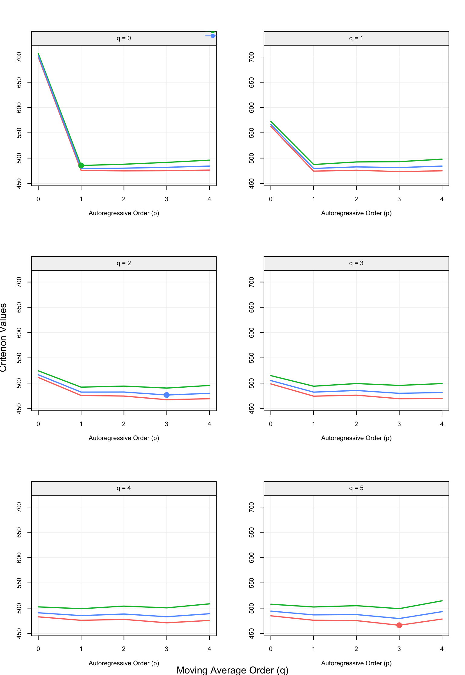
Figure 4.44: Values of the three model selection criteria for all possible candidate models included in an ARMA(4,5) model.
##
## Call:
## arima(x = xt, order = c(3, 0, 5), include.mean = include.mean)
##
## Coefficients:
##           ar1     ar2     ar3     ma1     ma2      ma3      ma4      ma5
##       -0.4939  0.3748  0.8625  1.4987  0.7951  -0.4955  -0.5172  -0.2575
## s.e.   0.0531  0.0635  0.0519  0.1301  0.2081   0.1869   0.1638   0.0862
##       intercept
##          0.1406
## s.e.     0.3949
##
## sigma^2 estimated as 0.5441: log likelihood = -223.08, aic = 466.15select(ARMA(4,5), Xt)From the selection procedure it would appear that the BIC criterion selects a simple AR(1) model for the annual copper time series while the AIC selects an ARMA(3,5) model. This reflects the properties of these two criteria since the BIC usually selects lower order models (e.g. it can under-fit the data) while the AIC usually does the opposite (e.g. it can over-fit the data). As expected, the HQ criterion lies somewhere inbetween the two previous criteria and selects an ARMA(3,2) model.
In order to decide which of these models to use in order to describe or predict the time series, one could estimate the MAPE for these three selected models.
##               MAPE       SD
## AR(1)     15.74291 1.747938
## ARMA(3,2) 16.97668 1.918485
## ARMA(3,5) 20.73869 1.619907
##
## MAPE suggests: AR(1)evaluate(list(AR(1), ARMA(3,2), ARMA(3, 5)), Xt, criterion = "MAPE", start = 0.5)Based on the MAPE, we would probably choose the AR(1) model but, considering the standard deviations of the empirical MAPE, the ARMA(3,2) appears to be a close enough candidate model. To obtain further information to choose a final model, one could check the behaviour of the residuals from these two models.
model_copper_ar1 = estimate(AR(1), Xt)
check(model_copper_ar1)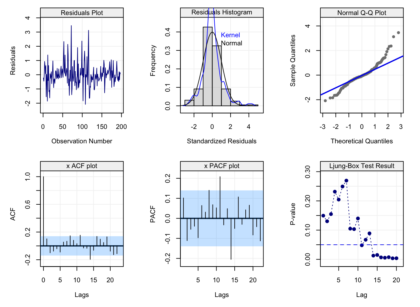
Figure 4.45: Diagnostic plots for the residuals of a fitted AR(1) to the annual copper prices.
model_copper_arma32 = estimate(ARMA(3,2), Xt)
check(model_copper_arma32)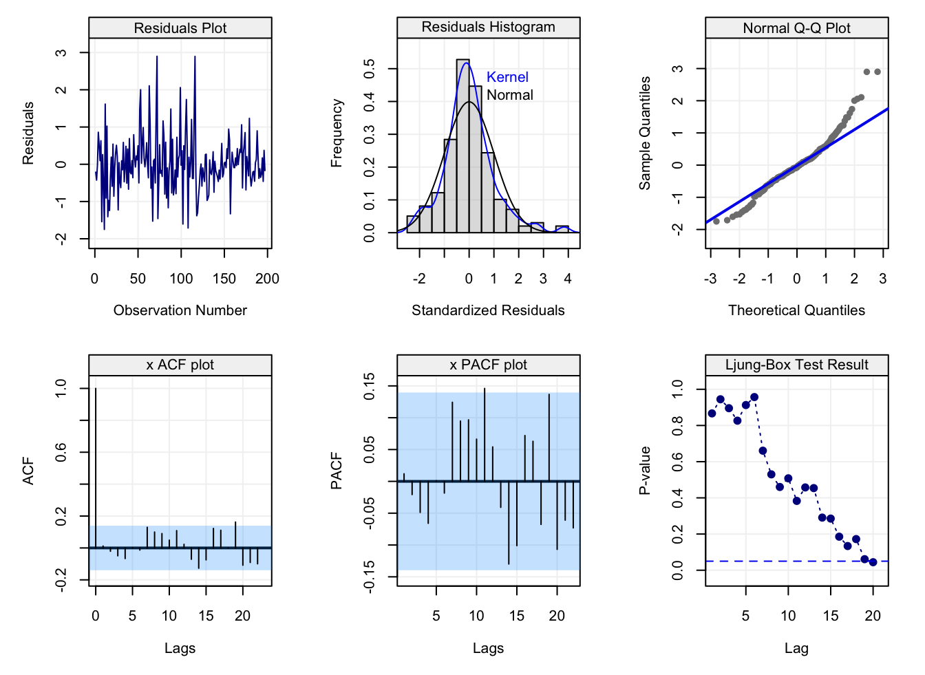
Figure 4.46: Diagnostic plots for the residuals of a fitted ARMA(3,2) to the annual copper prices.
From the two diagnostic plots we can see that the residuals from the AR(1) appear to preserve a certain degree of dependence (aside from large deviations from the normality assumption which, nevertheless, is not necessarily required). On the other hand, the residuals from the ARMA(3,2) have an overall better behaviour and, if one were to choose a unique model for this data, the ARMA(3,2) model would appear to be a good candidate.
4.8 ARIMA Models ⚠️
As we saw in the introduction to this book (and in various sections throughout it), a time series can be made of two components: a deterministic (non-stationary) component and a stochastic component. The latter component has been the main focus of this book where different classes of time series models have been studied assuming that this stochastic component respects certain properties (i.e. stationarity). For the former component (i.e. the deterministic component) we assume that we are able to explain non-stationary behaviours such as trends and seasonality via regression-type methods which include time-related covariates.
However, there are non-stationary behaviours that can be addressed without the need for estimation procedures to make a time series stationary. In fact, estimating parameters to remove deterministic components in the data adds uncertainty when modelling the time-dependent stochastic component since the residuals from the previous fitting are only an approximation of the stochastic component and may be a biased representation of the time series if the model used to fit the deterministic component is misspecified. Considering the possible drawbacks when using regression techniques to explain the deterministic components, we have already seen a technique that can be used to remove non-stationary components without the need for regression and this was based on the use of the backshift operator \(B\). The latter consists in a \(d\)-order differencing defined as:
\[\delta^d X_t = (1 - B)^d X_t.\] We have already seen some examples where a first-order difference (\(d=1\)) of a non-stationary time series can make the time series stationary. Indeed, a time series with a linear drift and/or a random walk can be made stationary by taking a first difference.
Example 4.22 For example, consider the model
\[X_t = \Delta + X_{t-1} + W_t,\] where \(\Delta\) is a drift constant and \(W_t \overset{iid}{\sim} WN(0, \sigma^2)\). A first difference of this process delivers:
\[\delta X_t = X_t - X_{t-1} = \Delta + W_t,\]
that is a stationary process with \(E[\delta X_t] = \Delta\) and \(Cov(\delta X_{t+h}, \delta X_t) = \sigma^2\) for \(h = 0\) and zero otherwise.A first-order difference can therefore remove linear trends in a time series but, if the non-stationary component of a time series has other behaviours, higher order differences can allow to make the series stationary.
Example 4.23 For example, take the following process:
\[X_t = \beta_0 + \beta_1 t + \beta_2 t^2 + Y_t,\] where \((Y_t)\) is a stationary time series. If we took the first difference of this time series we would obtain
\[\begin{align*} \delta X_t &= X_t - X_{t-1}\\ & = (\beta_0 + \beta_1 t + \beta_2 t^2 + Y_t) - (\beta_0 + \beta_1 (t-1) + \beta_2 (t-1)^2 + Y_{t-1}) \\ & = \beta_1 + \beta_2 (2t - 1) + \delta Y_t . \end{align*}\]This time series is not stationary either since its expectation depends on time. However, let us take the second difference:
\[\begin{align*} \delta^2 X_t &= \delta X_t - \delta X_{t-1}\\ & = (\beta_1 + \beta_2 (2t - 1) + \delta Y_t) - (\beta_1 + \beta_2 (2(t-1) - 1) + \delta Y_{t-1}) \\ & = \beta_2 2 + \delta^2 Y_t, \end{align*}\] which is now a stationary process with \(E[\delta^2 X_t] = 2 \beta_2\) and covariance function of \(\delta^2 Y_t\) which is a stationary process by definition.Therefore, if the time-dependent expectation of a time series can be explained by a \(d^{th}\)-order polynomial (i.e. \(\sum_{j=0}^d \beta_j t^j\)), the \(d^{th}\)-order difference of this time series will be stationary. There are many other non-stationary time series that can be made stationary in this manner (e.g. stochastic trend models).
Based on the properties of differencing, we can define the class of ARIMA(\(p\),\(d\),\(q\)) models as follows.
Based on this, the drift plus random walk described earlier would correspond to an ARIMA(0,1,0) since the first difference of the process delivers a white noise model with non-zero constant mean. To better illustrate the properties of these processes, let us consider the following ARIMA(2,1,1) model where \((X_t)\) is such that:
\[\delta X_t - 0.9 \delta X_{t-1} + 0.6 \delta X_{t-2} = 0.5 W_{t-1} + W_t.\] Below is a simulated realization of the time series of length \(T = 200\).
set.seed(123)
Xt = gen_gts(n = 200, model = ARIMA(ar = c(0.9, -0.6), i = 1, ma = 0.3, sigma2 = 0.5))
plot(Xt)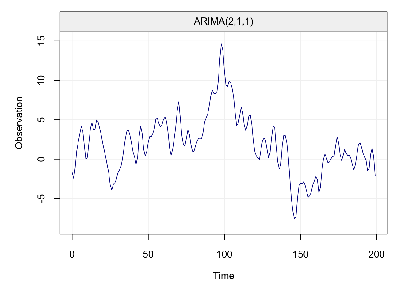
From the plot it is quite clear that the time series may not be stationary. For this reason, let us take the first difference of the time series and check if this operation allows us to visually satisfy the stationarity assumptions.
d_Xt = gts(diff(Xt))
plot(d_Xt)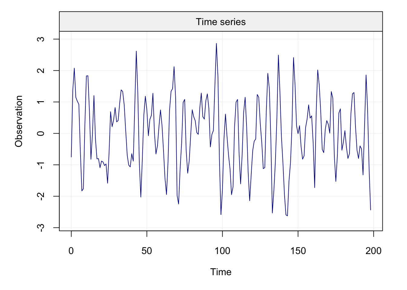
The first difference of the time series now appears to be stationary and, for this reason, let us analyse the ACF and PACF plots of this new time series.
corr_analysis(d_Xt)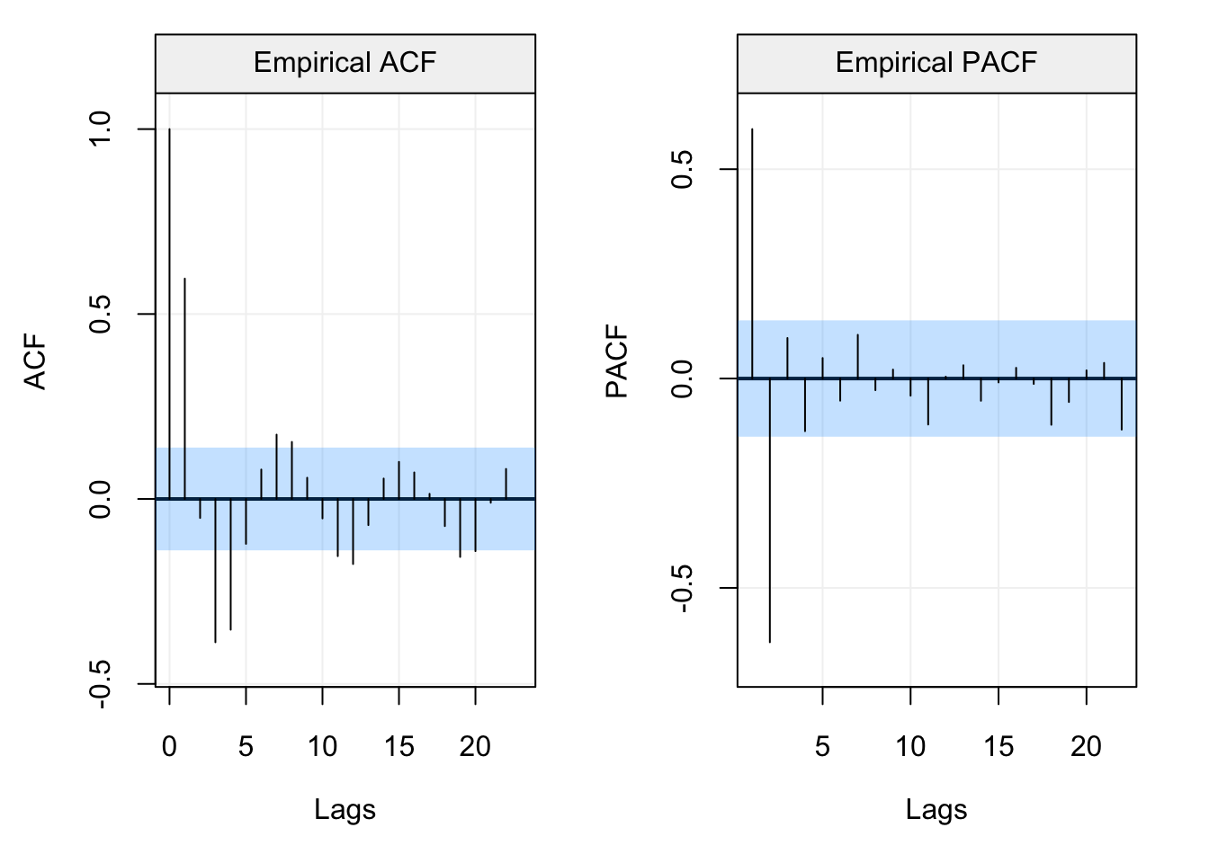
Both the ACF and PACF plots appear to have a decaying pattern with no clear cut-off points. Therefore, since these plots don’t perfectly fit either an AR(\(p\)) model or MA(\(q\)) model, we may consider an ARMA(\(p\),\(q\)) model for which the descriptive analysis provided by these plots is not necessarily helpful to understand the possible orders of the AR(\(p\)) and MA(\(q\)) components. For this reason, let us make use of the model selection criteria considering all models within an ARMA(3,3) for the process (\(\delta X_t\)).
select(ARIMA(3, 1, 3), Xt)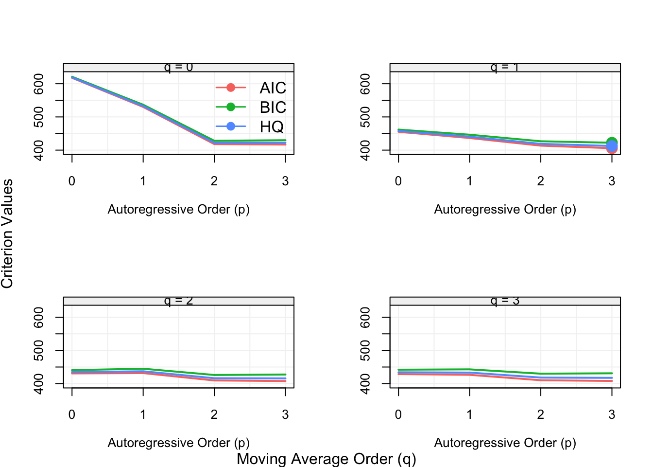
From the selection process we can see that all three criteria select the ARMA(2,1) model which is indeed the true model that generated the observed time series (i.e. more specifically an ARIMA(2,1,1) model). As in the previous sections, let us now consider also an example from some real data. The considered time series represents monthly sales of shampoo from 1901-1903 (available using the tsdl package) whose plot is shown below.
Xt = gts(as.numeric(subset(tsdl, description = "shampoo")[[1]]), start = 1901, freq = 12, name_ts = "Sales (Units)", data_name = "Monthly Shampoo Sales", name_time = "")
plot(Xt)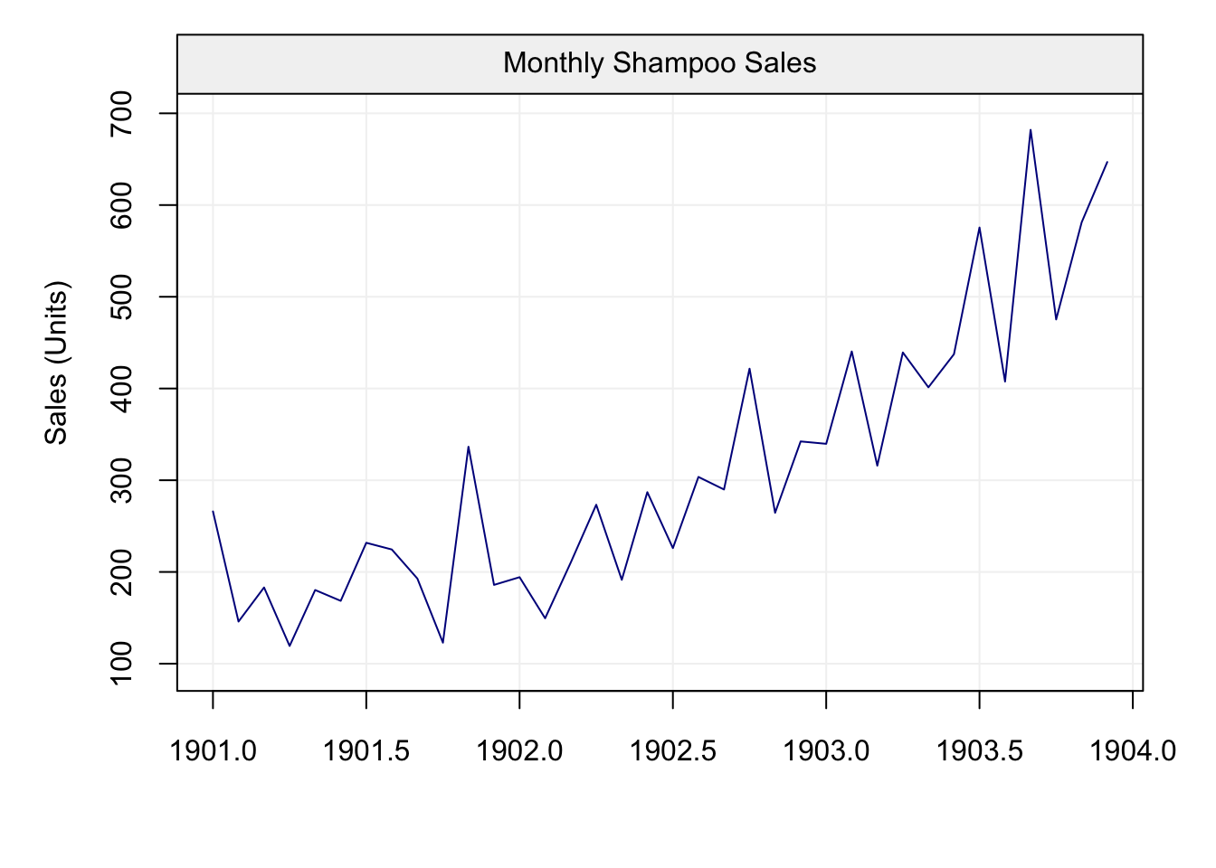
The plot of the time series shows a clear updward trend in the time series which could eventually be fitted by a (linear) regression. However, as discussed earlier, the use of estimation may not deliver “accurate” residuals that well represent the stochastic time series we want to model. Therefore, let us check if a first-order difference is capable of making the time series stationary.
d_Xt = gts(diff(Xt))

par(mfrow = c(2,1))
plot(d_Xt)
corr_analysis(d_Xt)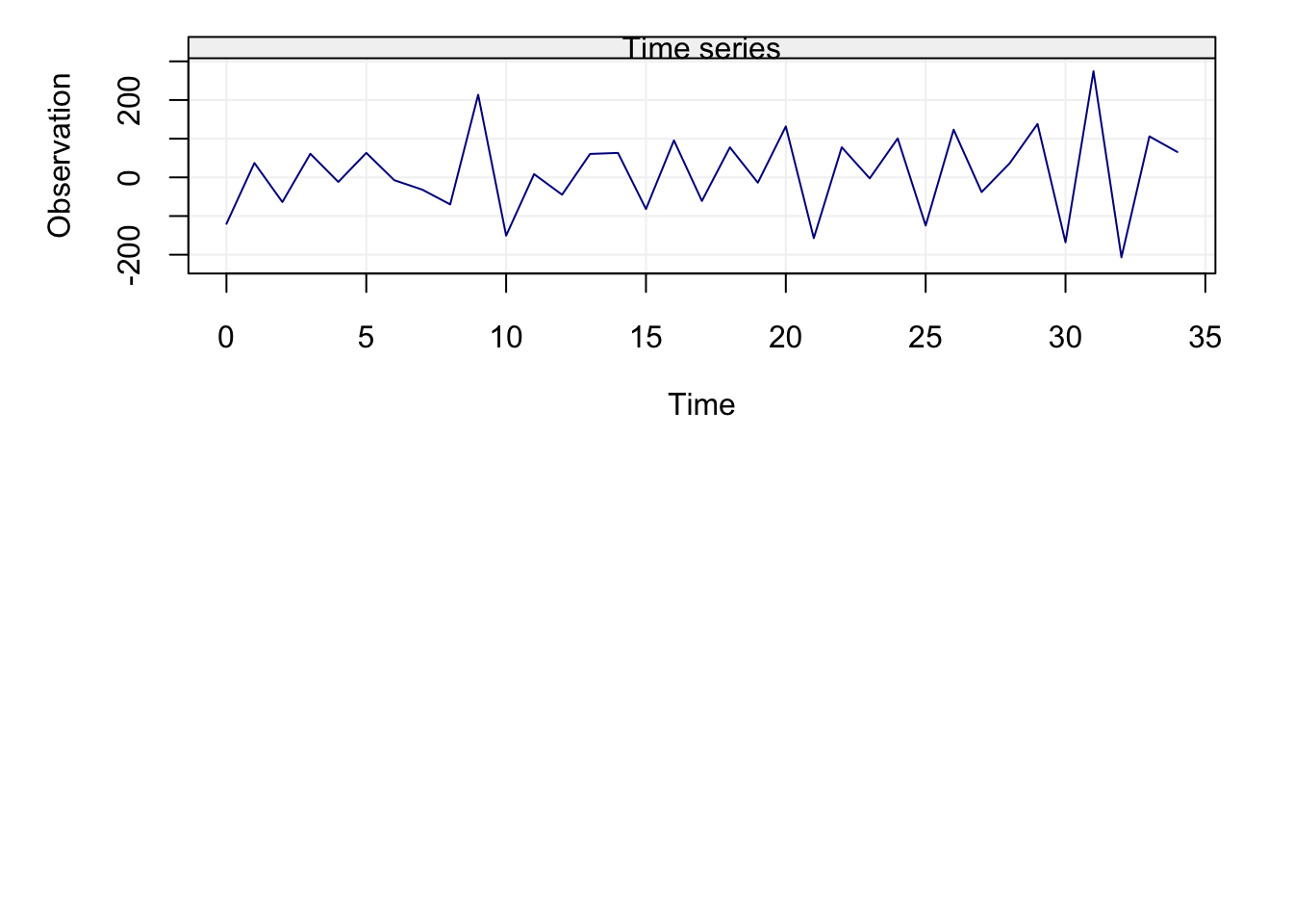
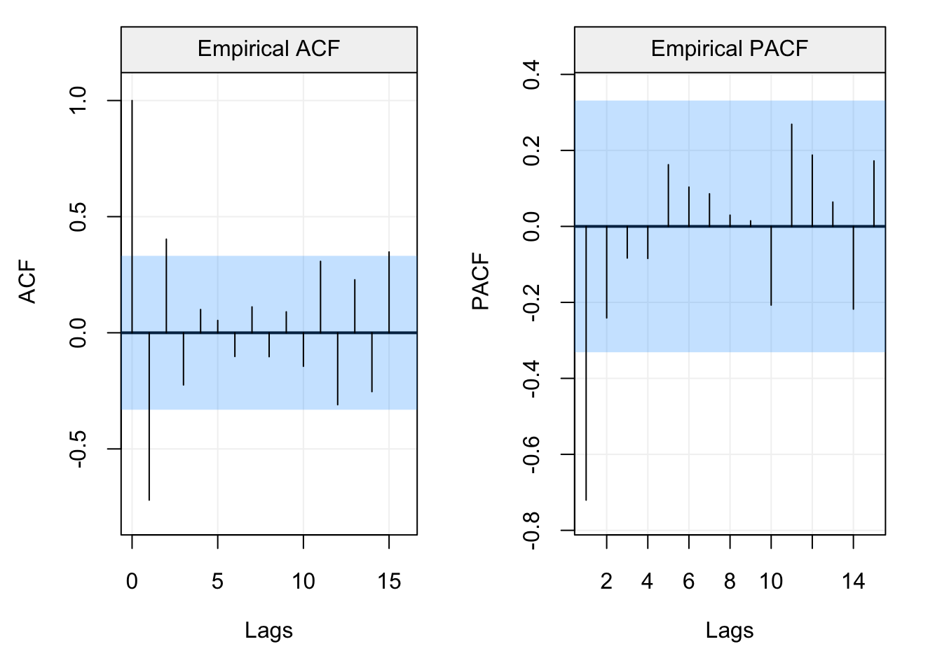
We can see how the first-differncing of the time series has allowed to make it apparently stationary so an ARIMA(\(p\),\(d\),\(q\)) model with \(d=1\) could be a good class of models to explain and predict the time series. The ACF and PACF plots would suggest a low order model since both the ACF and PACF become less significant starting from the first lags. For this reason, let us consider all candidate models included in an ARIMA(2,1,2) and evaluate them based on the model selection criteria.
select(ARIMA(2, 1, 2), Xt)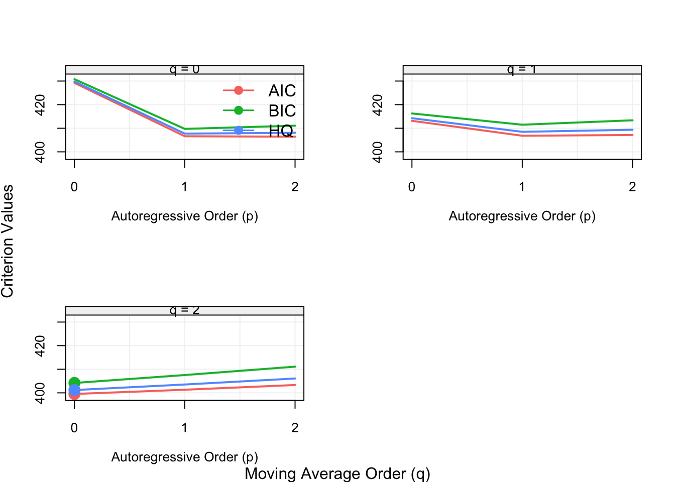
In this case, the most appropriate model would appear to be an ARIMA(0,1,2), meaning that an MA(2) model fitted to the first-difference of the original time series is the “best” to model the observed sales of shampoo.
4.9 SARIMA Models ⚠️
As seen in the previous section, ARMA models can be adapted in order to tackle different forms of non-stationary time series through the use of differencing, thereby delivering the class of ARIMA models. However, aside from non-stationarity, within different applied examples seen this far you may have noticed that many ACF (and PACF) plots denoted some forms of seasonality. Indeed, despite removing possible deterministic seasonal effects via regression techniques, it is often the case that some stochastic seasonal components appear in the (residual) time series. For this reason, the class of AR(I)MA models can be extended in order to take this seasonality into account thereby delivering the class of SARIMA models.
To introduce the more general class of SARIMA models, let us first consider the standard AR(1) model
\[X_t = \phi X_{t-1} + W_t,\] which explains the behaviour in time via the previous observation. Based on this model, for all time points the dependence on the past is explained by the previous observation at time \(t-1\). However, in the case of seasonal effects, this dependence on the past may be explained (also) by other lags \(t-s\), where \(s > 1\). For example, the following model
\[X_t = \phi X_{t-12} + W_t,\] is a first-order seasonal AR model with \(s = 12\) which is equivalent to an AR(12) model with \(\phi_i = 0\) for \(i = 1,...,11,\) and \(\phi_{12} \neq 0\). However, using an AR(12) model would be theoretically incorrect for this case (since there is no direct dependence on intermediate observations) and would be statistically inefficient to estimate and, consequently, the definition of a seasonal component is more appropriate. In fact, the definition of \(s = 12\) for the above example is typically the case of time series for economic or ecological phenomena where there can be a dependence between the same months.
Having justified the need for the extension to SARIMA models, let us more formally define this class of models starting from the example provided above.
Definition 4.12 (Seasonal Autoregressive Model of Order 1) A sesaonal autoregressive model of order 1 is defined as follows:
\[X_t = \Phi X_{t-s} + W_{t} \Leftrightarrow (1 - \Phi B^{s}) X_t = W_t\]
The model would have the following properties:
- \[\mathbb{E}[{X_t}] = 0\]
- \[\gamma(0) = \text{Var}\left[X_t\right] = \frac{\sigma^2}{1-\Phi^2}\]
- \[\rho(h) = \begin{cases} 1 &\text{ if } h = 0\\ \Phi^{\left|h\right|} &\text{ if } h = \pm \, s \cdot k, \, k = 1, 2, \cdots\\ 0 &\text{ otherwise. } \end{cases}\]
One aspect to underline at this point is the different notation used to explain seasonal dependence. Indeed, for standard AR(\(p\)) models the notation for autoregressive parameters in this book is \(\phi_i\) while for the seasonal dependence we have \(\Phi_i\). This is because a model can contain both standard AR(\(p\)) components (i.e. direct dependence on observations between \(t\) and \(t-p\)) as well as seasonal components where direct dependence can occur with observations at lags \(s > p\) (with no direct dependence on observations between \(t-p\) and \(t-s\)).
Keeping in mind the need for this additional notation, we can now define the first-order seasonal moving average process.
Definition 4.13 (Seasonal Moving Average of Order 1) A seasonal moving average model of order 1 is defined as follows:
\[X_t = W_t + \Theta W_{t-s} \Leftrightarrow X_t = (1 - \Theta B^{s}) W_t\]
\[\gamma(h) = \begin{cases} \left({1+\Theta^2}\right)\sigma^2 &\text{ if } h = 0 \\ \Theta \sigma^2 &\text{ if } h = \pm \, s \cdot k, \, k = 1, 2, \cdots \\ 0 &\text{ otherwise .} \\ \end{cases}\]
Therefore, a seasonal moving average is also defined in the same manner as a standard moving average model where the direct dependence is not strictly on the immediately adjacent past observations. Following the same logic, we can therefore define the seasonal equivalent of the autoregressive and moving average operators.
Definition 4.14 (Seasonal Autoregressive Operator) Similarly, to the regular autoregressive operator, the seasonal autoregressive operator is defined as:
\[\Phi_P(B^S) = 1 - \Phi_1 B^S - \Phi_2B^{2S} - \cdots - \Phi_PB^{PS}\]Definition 4.15 (Seasonal Moving Average Operator) The seasonal moving average operator is defined as:
\[\Theta_Q(B^S) = 1 + \Theta_1 B^S + \Theta_2B^{2S} + \cdots + \Theta_QB^{QS}\]In these cases, \(P\) and \(Q\) play the same role as the \(p\) and \(q\) orders for ARMA(\(p\),\(q\)) models thereby determining how far into the past the direct seasonal dependence is present. Given this notation, we can define a pure seasonal ARMA model.
Definition 4.16 (Pure Seasonal ARMA Model) A pure Seasonal ARMA model is defined as:
\[\Phi_P(B^S) X_t = \Theta_Q(B^S) W_t\]The above model therefore considers all direct seasonal dependencies without any components of standard ARMA models which can nevertheless be included to deliver a general SARMA model. Indeed, the more general SARMA model is defined as follows.
Definition 4.17 (Seasonal ARMA Model) Seasonal Autoregressive Moving Average models are often referred to with the notation \(ARMA(p, q)\times(P, Q)_{S}\) which indicates the following model:
\[\Phi_p \left({B^S}\right) \phi\left(B\right) X_t = \Theta_Q \left({ B^S }\right) \theta \left({ B }\right) W_t\]As you can notice, the standard autoregressive and moving average operators have now been added to the previous definition of pure seasonal ARMA models. Hence, as mentioned above, these models allow for different forms of direct dependence between observations and innovation (white) noise. Let us consider an example to understand the structure and properties of these models.
Example 4.24 (Mixed Seasonal Model) Consider the following time series model that contains both a seasonal term and a standard ARMA component:
\[X_t = \Phi X_{t-12} + \theta W_{t-1} + W_t, \,\,\, \left| \Phi \right| < 1, \,\, \left| \theta \right| < 1,\]
where \(W_t \sim WN(0, \sigma^2)\). Based on the previously defined notation, we can refer to this model as an \(ARMA(0,1)\times(1, 0)_{12}\) model. The properties of this model can be derived as follows:
\[\text{Var}\left( {{X_t}} \right) = {\Phi ^2} \text{Var} \left( {{X_{t - 12}}} \right) + {\sigma ^2} + {\theta ^2}{\sigma ^2} \]
Based on the parameter definitions, we know that this process is stationary (causal and invertible) and therefore \(\text{Var} \left( {{X_t}} \right) = \text{Var} \left( {{X_{t - 12}}} \right) = \gamma \left( 0 \right)\). Using this information we can derive the following:
\[\begin{align} \gamma \left( 0 \right) &= \frac{{{\sigma ^2}\left( {1 + {\theta ^2}} \right)}}{{1 - {\Phi ^2}}} \\[0.5cm] \gamma \left( 1 \right) &= \text{cov}\left( {{X_t},{X_{t - 1}}} \right) = \text{cov}\left( {\Phi {X_{t - 12}} + {W_t} + \theta {W_{t - 1}},{X_{t - 1}}} \right) \notag \\[0.2cm] &= \Phi \text{cov}\left( {{X_{t - 12}},{X_{t - 1}}} \right) + \underbrace {\text{cov}\left( {{W_t},{X_{t - 1}}} \right)}_{ = 0} + \theta \text{cov}\left( {{W_{t - 1}},{X_{t - 1}}} \right) \notag \\ &= \Phi \gamma \left( {11} \right) + \theta {\sigma ^2} \end{align}\]Then, for \(h > 1\) we have
\[\begin{align} \gamma \left( h \right) &= \text{cov}\left( {{X_t},{X_{t - h}}} \right) = \text{cov}\left( {\Phi {X_{t - 12}} + {W_t} + \theta {W_{t - 1}},{X_{t - h}}} \right) \notag \\[0.2cm] &= \Phi \text{cov}\left( {{X_{t - 12}},{X_{t - h}}} \right) \notag \\[0.2cm] &= \Phi \gamma \left( {h - 12} \right) \\ \end{align}\] Based on the above properties, we can show that the autocovariance will not be equal to zero for lags \(h\) that lie within the seasonal dependence structure. More specifically, let us use the last general definition of the autocovariance and, based on the symmetry of the autocovariance (i.e. \(\gamma (h) = \gamma(-h)\)), derive the explicit form for the autocovariance at lag \(h = 1\): \[\begin{equation} \gamma \left( 1 \right) = \Phi \gamma \left( {11} \right) + \theta {\sigma ^2} = {\Phi ^2}\gamma \left( 1 \right) + \theta {\sigma ^2} \end{equation}\]Based on the above equality we have:
\[\gamma \left( 1 \right) = \frac{{\theta {\sigma ^2}}}{{1 - {\Phi ^2}}}.\]
When the lag does not lie within the seasonal dependence structure the autocovariance will be zero. Consider, for example, the autocovariance at lag \(h=2\): \[\begin{align} \gamma \left( 2 \right) &= \text{cov} \left( {{X_t},{X_{t - 2}}} \right) = \operatorname{cov} \left( {\Phi {X_{t - 12}} + {W_t} + \theta {W_{t - 1}},{X_{t - 2}}} \right) \notag \\[0.2cm] &= \Phi \text{cov} \left( {{X_{t - 12}},{X_{t - 2}}} \right) = \Phi \gamma \left( {10} \right) = {\Phi ^2}\gamma \left( 2 \right). \end{align}\]Again, based on the above equality it can easily be seen that
\[\gamma \left( 2 \right) \left(1 - {\Phi ^2}\right) = 0 \,\, \Rightarrow \,\, \gamma \left( 2 \right) = 0\].
In this example, the same would hold for:
\[\begin{equation} \gamma \left( 3 \right) = \gamma \left( 4 \right) = \cdots = \gamma \left( 10 \right) = 0. \end{equation}\] Following these results, the general autocovariance of this model can be summarized as follows: \[\begin{align*} \gamma \left( {12h} \right) &= {\Phi ^h}\gamma \left( 0 \right) &h = 0, 1, 2, \ldots \\[0.2cm] \gamma \left( {12h + 1} \right) &= \gamma \left( {12h - 1} \right) = {\Phi ^h}\gamma \left( 1 \right) &h = 0, 1, 2, \ldots \\[0.2cm] \gamma \left( {h} \right) &= 0 &\text{otherwise} \end{align*}\]The autocorrelation function is easily derived from the above autocovariance structure and is given by:
\[\begin{align*} \rho \left( {12h} \right) &= {\Phi ^h} & h = 0, 1, 2, \ldots \\ \rho \left( {12h - 1} \right) &= \rho \left( {12h + 1} \right) = \frac{\theta }{{1 + {\theta ^2}}}{\Phi ^h} & h = 0, 1, 2, \ldots \\ \rho \left( h \right) &= 0 & \text{otherwise} \\ \end{align*}\]Given these derivations, let us verify what the estimated ACF of the above model looks like and, for this reason, we simulate a time series of length \(T = 10^4\) from an \(ARMA(0,1)\times(1, 0)_{12}\) model with \(\theta = -0.8\) and \(\Phi = 0.95\).
model = SARIMA(ar=0, i=0,ma=-0.8, sar=0.95, si = 0 , sma = 0, s = 12)
Xt = gen_gts(10e4, model)
plot(auto_corr(Xt, lag.max = 40))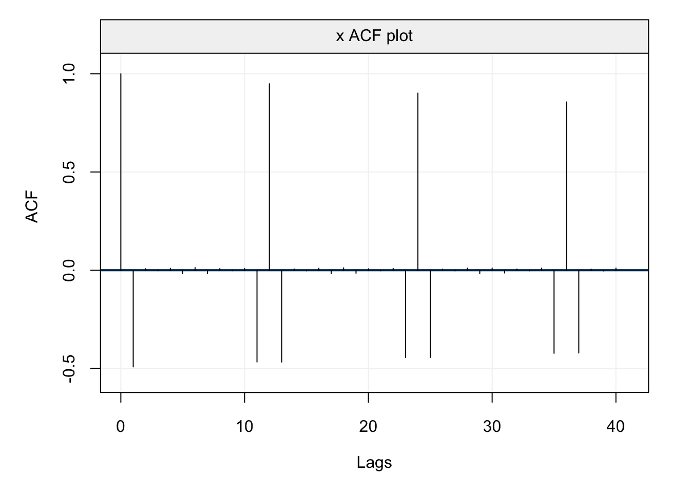
From the plot we can see how the autocorrelation is highly significant at each lag \(12 h\) as well as all adjacent lags \(12 h \pm 1\). This corresponds to what is expected from the autocorrelation structure of the model whose autocovariance structure we derived above.
Having provided a brief overview of how to derive and study the autocovariance (and autocorrelation) structure of these models, let us now verify how we can classify a time series model as a Seasonal ARMA. To better explain this, let us again consider the model whose autocovariance we have just studied.
Example 4.25 (Classifying a Seasonal ARMA) Returning to our previous example, we can see that the time series follows an \(ARMA(0,1)\times(1,0)_{12}\) process by rearranging the terms as follows.
\[\begin{align*} {X_t} &= \Phi {X_{t - 12}} + {W_t} + \theta {W_{t - 1}} \hfill \\[0.2cm] {X_t} - \Phi {X_{t - 12}} &= {W_t} + \theta {W_{t - 1}} \hfill \\[0.2cm] \underbrace {\left( {1 - \Phi {B^{12}}} \right)}_{{\Phi _1}\left( {{B^{12}}} \right)}\underbrace 1_{\phi \left( B \right)}{X_t} &= \underbrace 1_{{\Theta _Q}\left( B \right)}\underbrace {\left( {1 - \theta B} \right)}_{\theta \left( B \right)}{W_t} \hfill \\ \end{align*}\]For this model we can see how the autoregressive operator (\(\phi(B)\)) and the seasonal moving average operator (\(\Theta_Q(B)\)) are included but, for this model, are simply equal to one. With the information provided, we can now finally define the most general class of models presented in this chapter.
Definition 4.18 (Seasonal ARIMA Model) The Seasonal Autoregressive Integrated Moving Average model is denoted as \(ARIMA(p, d, q)\times(P, D, Q)_S\) and defined as:
\[\Phi_P \left({B^S}\right) \phi\left(B\right) \, \delta^D_S \, \delta^d X_t = \Theta_Q \left({ B^S }\right) \theta \left({ B }\right) W_t\]
where \(\delta^d = \left({1-B}\right)^d\) and \(\delta^D_S = \left({1-B^S}\right)^D\).You can notice that the definition of this model is quite complex but delivers an extremely flexible class of models that allows to describe (and predict) a wide range of time series with different forms of non-stationarity and seasonality. Indeed, aside from the previous forms of non-stationarity addressed by ARIMA models (\(\delta^d\)), these models also allow to address the same forms of non-stationarity within the seasons (\(\delta^D_S\)) in addition to the different dependence structures made available by SARMA models. However, the increased complexity of these models comes at a certain cost. For example, classifying a time series model as a SARIMA model becomes a slightly more lengthy procedure.
Example 4.26 (Classifying a SARIMA) Consider the following time series:
\[{X_t} = {X_{t - 1}} + {X_{t - 12}} - {X_{t - 13}} + {W_t} + \theta {W_{t - 1}} + \Theta {W_{t - 12}} + \Theta \theta {W_{t - 13}}.\]
We can rearrange the terms of this model in order to classify it as a SARIMA model as follows:
\[\begin{align} {X_t} - {X_{t - 1}} - {X_{t - 12}} + {X_{t - 13}} &= {W_t} + \theta {W_{t - 1}} + \Theta {W_{t - 12}} + \Theta \theta {W_{t - 13}} \hfill \\[0.2cm] \left( {1 - B - {B^{12}} + {B^{13}}} \right){X_t} &= \left( {1 + \theta B + \Theta {B^{12}} + \theta \Theta {B^{13}}} \right){W_t} \end{align}\]At this point the trick is to try and detect if the polynomials of the backshift operator \(B\) can be factorized into simple differencing polynomials and/or seasonal and standard ARMA polynomials. In this case, it is possible to show this as follows:
\[\underbrace {\left( {1 - {B^{12}}} \right)}_{{\delta_{12}^1}}\underbrace {\left( {1 - B} \right)}_{\delta^1} {X_t} = \underbrace {\left( {1 + \Theta {B^{12}}} \right)}_{{\Theta _Q}\left( {{B^S}} \right)}\underbrace {\left( {1 + \theta B} \right)}_{\theta \left( B \right)}{W_t}, \]
Indeed, the polynomials for the observations \(X_t\) do not depend on any parameters and are therefore simply differencing polynomials while those for the innovation noise both depend on parameters and therefore constitute the seasonal and standard moving average polynomials. Based on this final form, we can conclude that the initial time series model can be classified as a SARIMA model which can be denoted as \(ARIMA(0,1,1)\times(0,1,1)_{12}\).Another additional problem due to the complexity of these models is identifying the order of the different terms \(p, d, q, P, D, Q, s\). In fact, as we saw in the previous sections, this is already not straightforward for standard ARMA models and becomes even more challenging for SARIMA models. The first approach is to understand if the time series is stationary and, if not, try and visually assess whether a standard and/or seasonal differencing allows to make the time series stationary (thereby defining \(d\) and/or \(D\)). Once this is done, one can use the ACF and PACF plots to check the behaviour of the autocovariance and eventually detect forms of stochastic seasonality with peaks at regular lagged intervals (thereby defining \(s\)). Finally, the definition of the terms \(p, q, P, Q\) is usually done via prior knowledge of the phenomenon underlying the time series data or via model selection criteria for which one determines a (large) model within which to select among all possible candidates included within this model.
The procedure to modelling data always has a subjective input and two (or more) different models can be equally effective in describing and/or predicting a given time series. Therefore, as for all applied examples in this book, we will now provide insight to one among many possible ways to fit a model to a given time series. For this reason, let us consider the monthly water levels of Lake Erie from 1921 to 1970.
Xt = gts(as.numeric(subset(tsdl, description = "Erie")[[1]]),
    start = 1921, freq = 12, name_ts = "Water Levels",
    data_name = "Monthly Lake Erie Levels", name_time = "")
plot(Xt)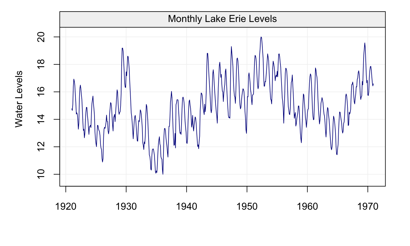
Figure 4.47: Monthly Water Levels of Lake Erie between 1921 and 1970
We can see how the time series appears to fluctuate hinting that it may not be stationary. Moreover, knowing that the time series represents a natural phenomenon observed over months, it could be reasonable to think that the weather (and consequent water cycle) has an impact on the water levels thereby entailing some form of seasonality. Indeed, when looking at ACF and PACF plots of this data, it can be seen how there is a sinusoidal wave with peaks at lags 12 and 24 (and possibly further) indicating that there appears to be high correlation between the same months.
corr_analysis(Xt)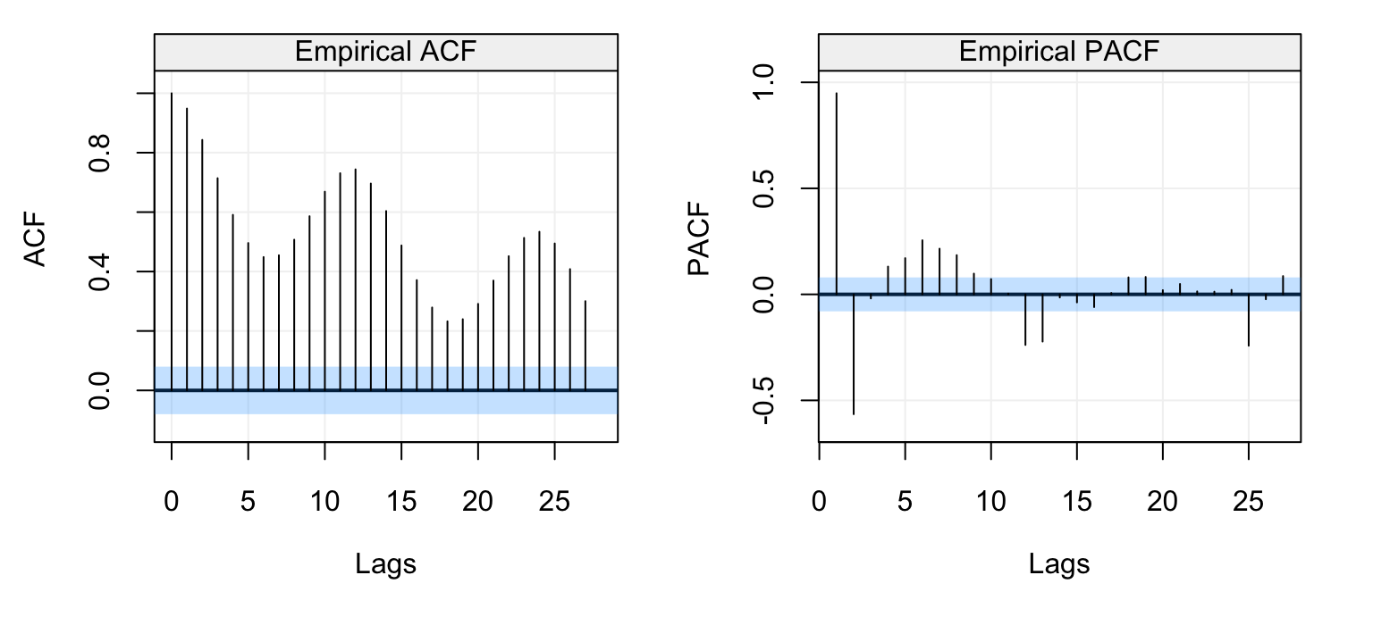
Figure 4.48: Empirical ACF (left) and PACF (right) of the Lake Erie time series data.
Considering the possible non-stationarity in the data, would differencing the time series make it stationary? And if so, which kind of differencing? Let us consider the first-order difference as well as a seasonal difference with \(s = 12\) (since that what appears in the ACF plot).
d_Xt = gts(diff(Xt))
d_s = gts(diff(Xt, lag = 12))
par(mfrow = c(2,1))
plot(d_Xt)
plot(d_s)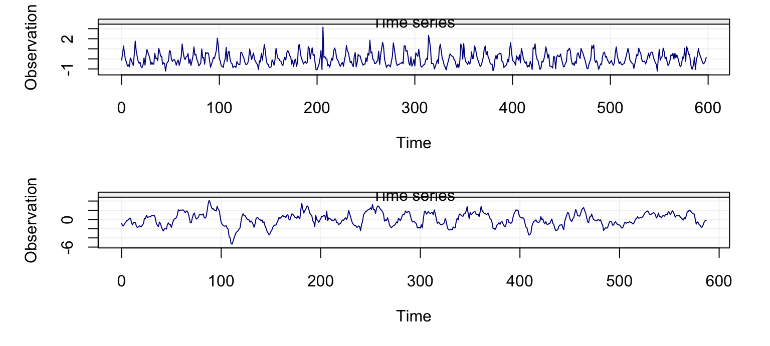
Figure 4.49: First difference (top) and difference at lag 12 (bottom) of the Lake Erie time series data.
We can see how both differencing approaches appear to make the resulting time series (reasonably) stationary. If we take a look at the ACF and PACF plots of the seasonal differencing, we can see how the ACF does not show clear seasonality anymore while some residual seasonality can be observed in the PACF plot.
corr_analysis(d_s)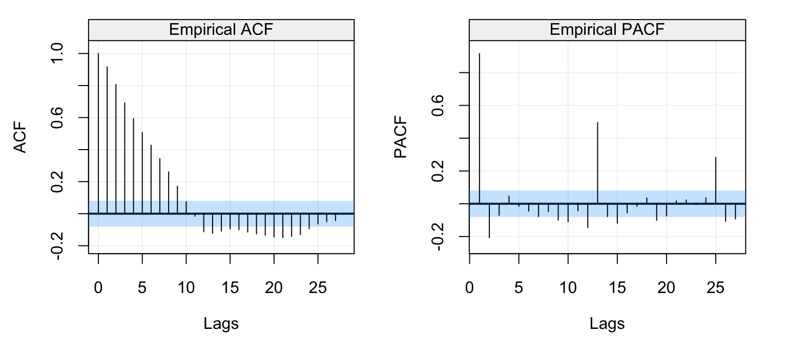
Figure 4.50: Empirical ACF (left) and PACF (right) of the seasonal difference (\(s = 12\)) of the Lake Erie time series data.
Since both differencings appear to do a good job in making the time series stationary, let us consider a SARIMA model with \(d=1\), \(D=1\) and \(s = 12\). Moreover, considering the structure of the ACF we could envisage using an AR(\(p\)) component in additional to some seaonsal components to address the residual seasonality in the PACF. Hence, let us estimate a SARIMA model defined as \(ARIMA(2,1,0)\times(1,1,1)_{12}\).
mod = estimate(SARIMA(ar = 2, i = 1, sar = 1, sma = 1, s = 12, si = 1), Xt, method = "mle")
check(mod)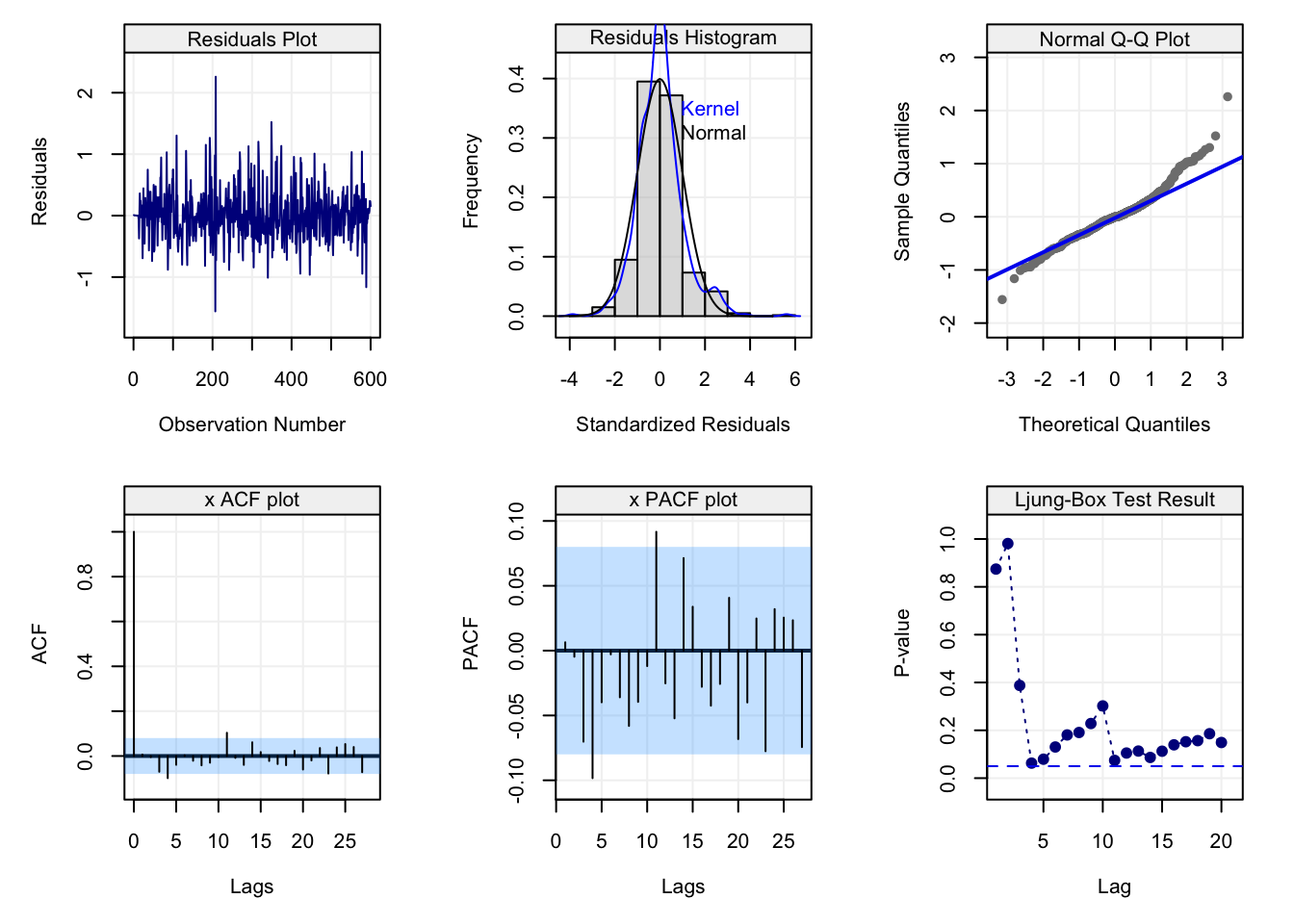
Based on the diagnostic plots, we can see that this model does a reasonably good job and could therefore be considered as a candidate model for explaining/predicting this time series. Supposing we were hydrologists who intend to plan the management of water resources over the next two years: we may therefore be interested in understanding/predicting the future behaviour of the lake’s water levels over the next 24 months. As for ARMA models, we can also predict using SARIMA models and, for this particular data and model, we obtain the following forecast.
predict(mod, n.ahead = 24)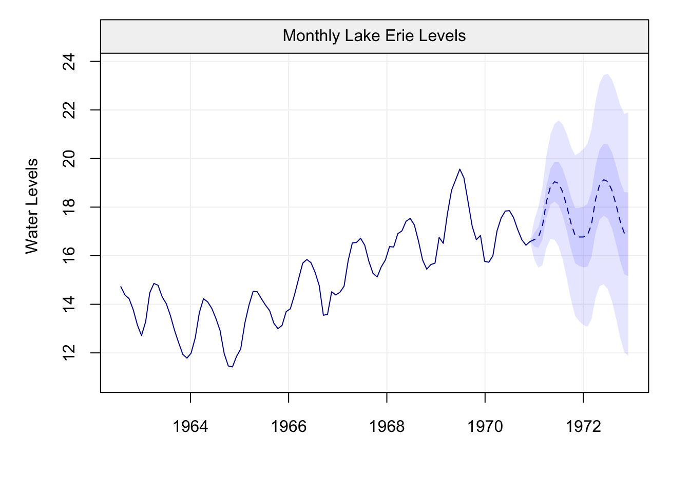
As you can see, the forecasted values (and confidence intervals) appear to reasonably follow the pattern of the observed time series confirming that the fitted model could be a possible candidate to consider for the considered time series data.
C Proofs
McQuarrie, Allan DR, and Chih-Ling Tsai. 1998. Regression and Time Series Model Selection. World Scientific.
Mallows, Colin L. 1973. “Some Comments on c P.” Technometrics 15 (4). Taylor & Francis Group: 661–75.
Akaike, Hirotugu. 1974. “A New Look at the Statistical Model Identification.” IEEE Transactions on Automatic Control 19 (6). Ieee: 716–23.
Schwarz, Gideon, and others. 1978. “Estimating the Dimension of a Model.” The Annals of Statistics 6 (2). Institute of Mathematical Statistics: 461–64.
Hannan, Edward J, and Barry G Quinn. 1979. “The Determination of the Order of an Autoregression.” Journal of the Royal Statistical Society. Series B (Methodological). JSTOR, 190–95.
Shibata, Ritei. 1980. “Asymptotically Efficient Selection of the Order of the Model for Estimating Parameters of a Linear Process.” The Annals of Statistics. JSTOR, 147–64.