B Robust Regression Methods
This appendix is largely based on the introduction to linear robust regression presented in Ronchetti (2006) and Duncan and Guerrier (2016). In these references it is stated that the vast majority of the statistical models employed in different fields going from finance to biology and engineering, for example, are parametric models. Based on these models, assumptions are made concerning the properties of the variables of interest (and the models themselves) and optimal procedures are derived under these assumptions. Among these procedures, the least squares and maximum likelihood estimators are well known examples that, however, are only optimal when the underlying statistical assumptions are exactly satisfied. If the latter case does not hold, then these procedures can become considerably biased and/or inefficient when there exist small deviations from the model. The results obtained by classical procedures can therefore be misleading when applied to real data (see e.g. Ronchetti (2006) and Huber and Ronchetti (2009)).
In order to address the problems arising from violated parametric assumptions, robust statistics can be seen as an extension to classical parametric statistics by directly considering the deviations from the models. Indeed, while parametric models may be a good approximation of the true underlying situation, robust statistics does not assume that the model is exactly correct. A robust procedure as stated in Huber and Ronchetti (2009) therefore should have the following features:
- It should efficiently estimate the assumed model.
- It should be reliable and reasonably efficient under small deviations from the model (e.g. when the distribution lies in a neighborhood of the assumed model).
- Larger deviations from the model should not affect the estimation procedure excessively.
A robust estimation method is a compromise with respect to these three features. This compromise is illustrated by Anscombe and Guttman (1960) using an insurance metaphor: “sacrifice some efficiency at the model in order to insure against accidents caused by deviations from the model”.
It is often believed that robust procedures may be avoided by using the following two-step procedure:
- Clean the data using some rule for outlier rejection.
- Apply classical optimal procedures on the “clean” data.
Unfortunately such procedures cannot replace robust methods as discussed in Huber and Ronchetti (2009) for the following reasons:
- It is rarely possible to seperate the two steps. For example, in a parametric regression setting, outliers are difficult to recognize without reliable (i.e. robust) estimates of the model’s parameters.
- The cleaned data will not correspond to the assumed model since there will be statistical errors of both kinds (false acceptance and false rejection). Therefore in general the classical theory is not applicable to the cleaned sample.
- Empirically, the best rejection procedures do not reach the performance of the best robust procedures. The latter are apparently superior because they can make a smoother transition between the full acceptance and full rejection of an observation using weighting procedures Hampel et al. (1987).
- Empirical studies have also shown that many of the classical rejection methods are unable to deal with multiple outliers. Indeed, it is possible that a second outlier “masks” the effect of the first so that neither are rejected.
Unfortunately the least squares estimator suffers from a dramatic lack of robustness. A single outlier can have an arbitrarily large effect on the estimated parameters. In order to assess the robustness of an estimator we first need to introduce an important concept, namely the influence function. This concept was introduced in Hampel (1968) and it formalizes the bias caused by one outlier. The influence function of an estimator represents the effect of an infinitesimal contamination at the point \(x\) or (\(\mathbf{x}\), \(y\)) in the regression setting) on the estimate, standardized by the mass of contamination. Mathematically, the influence function of the estimator \(T\) for the model \(F\) is given by:
\[\text{IF}(x| T, F) = \lim_{\varepsilon \rightarrow 0} \frac{T\left((1-\varepsilon) F + \varepsilon \Delta_x \right) - T\left(F\right)}{\varepsilon}\]
where \(\Delta_x\) is a probability measure which puts mass \(1\) at the point \(x\).
B.1 The Classical Least-Squares Estimator
The standard definition of the linear model is derived as follows. Let \({(\mathbf{x}_{i},y_{i}): i = 1, \ldots, n}\) be a sequence of independent identically distributed random variables such that:
\[y_{i} = \mathbf{x}_{i}^{T} {\boldsymbol{\beta}} + u_{i}\]
where \(y_{i} \in \mathbb{R}\) is the \(i\)-th observation, \(\mathbf{x}_{i} \in \mathbb{R}^{p}\) is the \(i\)-th row of the design matrix \(\mathbf{X} \in \mathbb{R}^{n\times p}\), \(\boldsymbol{\beta} \in \boldsymbol{\Theta} \subseteq \mathbb{R}\) is a p-vector of unknown parameters, \(u_{i} \in \mathbb{R}\) is the \(i\)-th error.
The least-squares estimator \(\hat{\boldsymbol{\beta}}_{LS}\) of \(\boldsymbol{\beta}\) can be expressed as an \(M\)-estimator1 Least-squares estimators are an example of the larger class of \(M\)-estimators. The definition of \(M\)-estimators was motivated by robust statistics which delivered new types of \(M\)-estimators. defined by the estimating equation:
\[\begin{equation} \sum_{i = 1}^{n} \left(y_{i} - \mathbf{x}_{i}^{T} \boldsymbol{\beta} \right)\mathbf{x}_{i} = 0. \tag{B.1} \end{equation}\]This estimator is optimal under the following assumptions:
- \(u_{i}\) are normally distributed.
- \(\mathbb{E}[u_{i}] = 0\) for \(i = 1, \ldots, n\).
- \(Cov(u_{1}, \ldots, u_{n}) = \sigma^2 \, \mathbf{I}_{n}\) where \(\mathbf{I}_{n}\) denotes the identity matrix of size \(n\).
In other words, least-squares estimation is only optimal when the errors are normally distributed. Small departures from the normality assumption for the errors results in considerable loss of efficiency of the least-squares estimator (see Hampel et al. (1987), Huber (1973) and Hampel (1973)).
B.2 Robust Estimators for Linear Regression Models
The “Huber estimator” introduced in Huber (1973) was one of the first robust estimation methods applied to linear models. Basically, this estimator is a weighted version of the least-squares estimate with weights of the form:
\[ w_{i} = \min \left(1,\frac{c}{|r_{i}|}\right) \]
where \(r_{i}\) is the \(i\)-th residual and \(c\) is a positive constant which controls the trade-off between robustness and efficiency.
Huber proposed an -estimator \(\hat{\boldsymbol{\beta}}_{H}\) of \(\boldsymbol{\beta}\) defined by the estimating equation:
\[ \sum_{i = 1}^{n} \psi_{c}\left(y_{i} - \mathbf{x}_{i}^{T} \boldsymbol{\beta} \right)\mathbf{x}_{i} = 0 \]
where \(\psi_{c}(\cdot)\) corresponds to Huber’s weight function
\[\begin{equation} w\left({x}\right) = \begin{cases} 1, &\text{if } \left|{x}\right| \le k \\ \frac{k}{\left|{x}\right|}, &\text{if} \left|{x}\right| > k \end{cases} \tag{B.2} \end{equation}\]and, thus, is defined as:
\[ \psi_{c}(r) = \left\{ \begin{array}{l l} r & \quad \\ c \cdot \text{sign}(r). & \quad \\ \end{array} \right. \]
However, the Huber estimator cannot cope with problems caused by outlying points in the design (or covariate) matrix \(X\). An estimator which was developed to address this particular issue is the one proposed by Mallows which has the important property that the influence function is bounded also for the matrix \(X\) (see Krasker (1980) for more details).
B.3 Applications of Robust Estimation
Having rapidly highlighted the theory of robustness, we now focus on the application of robust techniques in practical settings. Over the next three examples, estimation between classical or traditional methods will be compared with robust methods to illustrate the usefulness of using the latter techniques can have in specific scenarios.
Example B.1 Consider a simple linear model with Gaussian errors such as
\[\begin{equation} y_i = \alpha + \beta x_i + \varepsilon_i, \;\; \varepsilon_i \overset{iid}{\sim} \mathcal{N}(0,\sigma^2) \tag{B.3} \end{equation}\] for \(i = 1,...,n\). Next, we set the parameter values \(\alpha = 5\), \(\beta = 0.5\) and \(\sigma^2 = 1\) in order to simulate 20 observations from the above simple linear model where we define \(x_i = i\) for \(i = 1,...,20\). In the left panel of Figure B.1, we present the simulated observations together with the fitted regression lines obtained by least-squares and a robust estimation method. It can be observed that both lines are very similar and “close” to the true model given by \(y_i = 5 + 0.5 i\). Indeed, although the robust estimator pays a small price in terms of efficiency compared to the the least-squares estimator, the two methods generally deliver very “similar” results when the model assumption holds. On the other hand, the robust estimators provide (in general) far more reliable results when outliers are present in a data-set. To illustrate this behavior we modify the last observation by setting \(\varepsilon_{20} = -10\) (which is “extreme” under the assumption that \(\varepsilon_i \overset{iid}{\sim} \mathcal{N}(0,1)\)). The modified observations are presented in the right panel of Figure B.1 together with the fitted regression lines. In this case, the least-squares is strongly influenced by the outlier we introduced while the robust estimator remains stable and “close” to the true model.# Load robust library
library("robustbase")
# Set seed for reproducibility
set.seed(867)
# Sample size
n = 20
# Model's parameters
alpha = 5 # Intercept
beta = 0.5 # Slope
sig2 = 1 # Residual variance
# Construct response variable y
x = 1:n
y = alpha + beta*x + rnorm(n,0,sqrt(sig2))
# Construct "perturbed" verison of y
y.perturbed = y
y.perturbed[20] = alpha + beta*x[20] - 10
# Compute LS estimates
LS.y = lm(y ~ x)
LS.y.fit = coef(LS.y)[1] + coef(LS.y)[2]*x
LS.y.pert = lm(y.perturbed ~ x)
LS.y.pert.fit = coef(LS.y.pert)[1] + coef(LS.y.pert)[2]*x
# Compute robust estimates
RR.y = lmrob(y ~ x)
RR.y.fit = coef(RR.y)[1] + coef(RR.y)[2]*x
RR.y.pert = lmrob(y.perturbed ~ x)
RR.y.pert.fit = coef(RR.y.pert)[1] + coef(RR.y.pert)[2]*x
# Define colors
gg_color_hue <- function(n, alpha = 1) {
hues = seq(15, 375, length = n + 1)
hcl(h = hues, l = 65, c = 100, alpha = alpha)[1:n]
}
couleurs = gg_color_hue(6)
# Compare results based on y and y.perturbed
par(mfrow = c(1,2))
plot(NA, ylim = range(cbind(y,y.perturbed)), xlim = range(x),
main = "Uncontaminated setting", xlab = "x", ylab = "y")
grid()
points(x,y, pch = 16, col = couleurs[4])
lines(x, alpha + beta*x, col = couleurs[3], lty = 2)
lines(x, LS.y.fit, col = couleurs[5])
lines(x, RR.y.fit, col = couleurs[1])
legend("topleft",c("Observations","Estimated model (least-squares)",
"Estimated model (robust)", "True model"),
lwd = c(NA,1,1,1), col = couleurs[c(4,5,1,3)],
lty = c(NA,1,1,2), bty = "n", pch = c(16,NA,NA,NA))
plot(NA, ylim = range(cbind(y,y.perturbed)), xlim = range(x),
main = "Contaminated setting", xlab = "x", ylab = "y")
grid()
points(x[1:19],y.perturbed[1:19], pch = 16, col = couleurs[4])
points(x[20], y.perturbed[20], pch = 15, col = couleurs[6])
lines(x, alpha + beta*x, col = couleurs[3], lty = 2)
lines(x, LS.y.pert.fit, col = couleurs[5])
lines(x, RR.y.pert.fit, col = couleurs[1])
legend("topleft",c("Uncontamined observations", "Contamined observation",
"Estimated model (least-squares)", "Estimated model (robust)",
"True model"), lwd = c(NA,NA,1,1,1), col = couleurs[c(4,6,5,1,3)],
lty = c(NA,NA,1,1,2), bty = "n", pch = c(16,15,NA,NA,NA))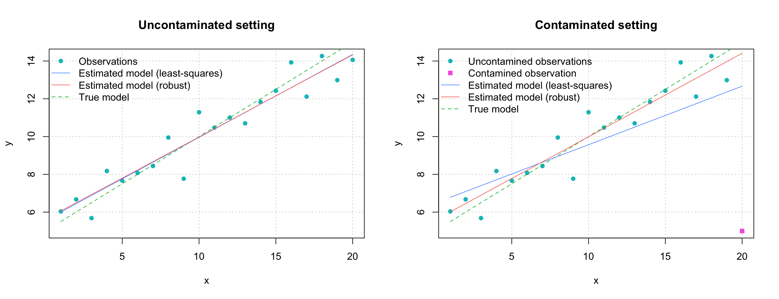
Figure B.1: Simulation Study Comparing Robust and Classical Regression Methodologies
# Number of bootstrap replications
B = 10^3

# Initialisation
coef.LS.cont = coef.rob.cont = matrix(NA,B,2)
coef.LS.uncont = coef.rob.uncont = matrix(NA,B,2)

# Start Monte-carlo
for (j in 1:2){
  for (i in seq_len(B)) {
   # Control seed
    set.seed(2*j*B + i)

    # Uncontaminated case
    if (j == 1){
      y = alpha + beta*x + rnorm(n,0,sqrt(sig2))
      coef.LS.uncont[i,] = as.numeric(lm(y ~ x)$coef)
      coef.rob.uncont[i,] = as.numeric(lmrob(y ~ x)$coef)
    }

    # Contaminated case
    if (j == 2){
      y = alpha + beta*x + rnorm(n,0,sqrt(sig2))
      y[20] = alpha + beta*x[20] - 10
      coef.LS.cont[i,] = as.numeric(lm(y ~ x)$coef)
      coef.rob.cont[i,] = as.numeric(lmrob(y ~ x)$coef)
    }
  }
}

# Make graph
colors = gg_color_hue(6, alpha = 0.5)
names = c("LS - uncont","Rob - uncont","LS - cont","Rob - cont")

par(mfrow = c(1,2))
boxplot(coef.LS.uncont[,1],coef.rob.uncont[,1],coef.LS.cont[,1],
        coef.rob.cont[,1], main = expression(alpha),
        col = colors[c(5,1,5,1)],
        cex.main = 1.5, xaxt = "n")
axis(1, labels = FALSE)
text(x = seq_along(names), y = par("usr")[3] - 0.15, srt = 45, adj = 1,
     labels = names, xpd = TRUE)

abline(h = alpha, lwd = 2)

boxplot(coef.LS.uncont[,2],coef.rob.uncont[,2],coef.LS.cont[,2],
        coef.rob.cont[,2], main = expression(beta),
        col = colors[c(5,1,5,1)],
        cex.main = 1.5, xaxt = "n")
axis(1, labels = FALSE)
text(x = seq_along(names), y = par("usr")[3] - 0.015, srt = 45, adj = 1,
     labels = names, xpd = TRUE)
abline(h = beta, lwd = 2)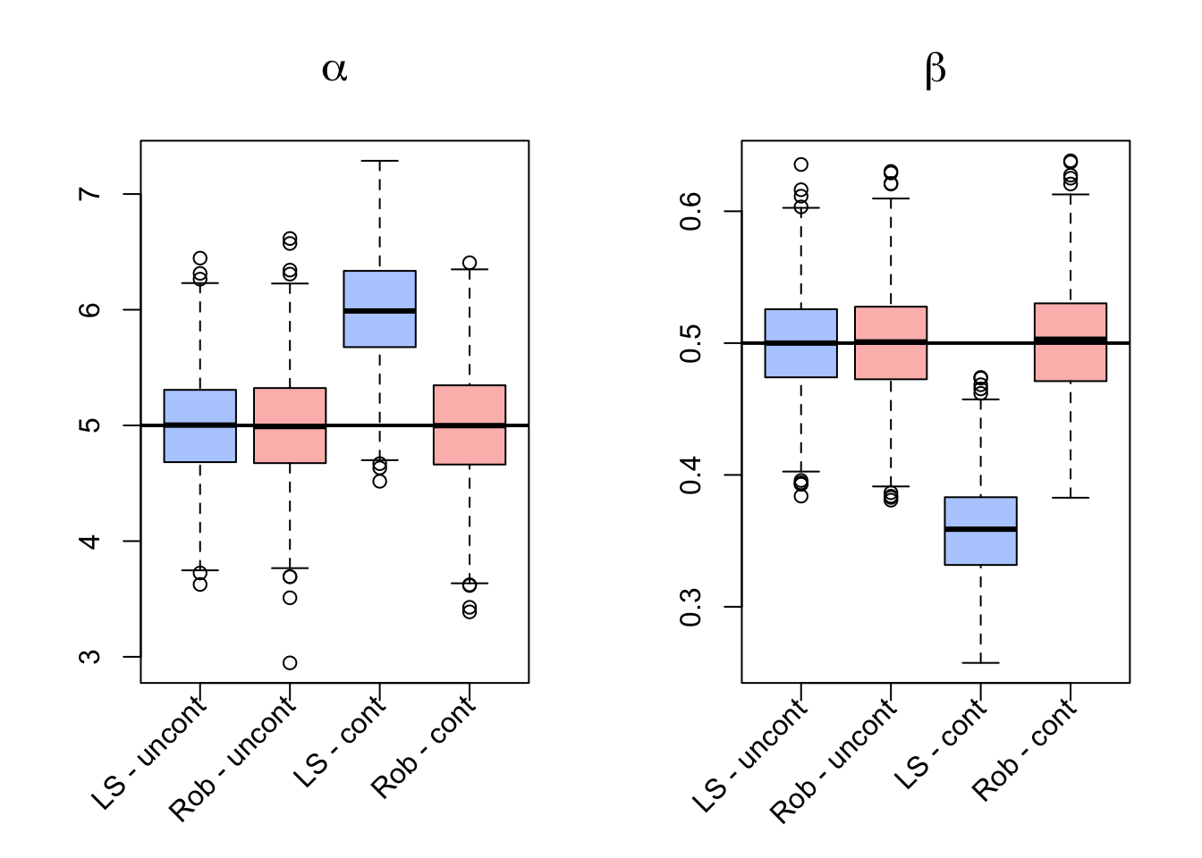
It can be seen that, as underlined earlier, that the estimations resulting from the two methods appear to be quite similar, with the robust estimator performing slightly less efficiently than the classical estimator. However, under the contaminated setting it is evident how the robust estimation procedure is not affected much by the outliers in the simulated data while the classical techniques appear to be highly biased. Therefore, if there appear to be outliers in the data, a robust estimation procedure may considered preferable. In fact, the results of the two estimations could be compared to understand if there appears to be some deviation from the model assumptions.
colors = gg_color_hue(6)
data(starsCYG, package = "robustbase")
par(mfrow = c(1,1))
plot(NA, xlim = range(starsCYG$log.Te) + c(-0.1,0.1),
     ylim = range(starsCYG$log.light),
     xlab = "Temperature at the surface of the star (log)",
     ylab = "Light intensity (log)")
grid()
points(starsCYG, col = colors[4], pch = 16)

LS = lm(starsCYG$log.light ~ starsCYG$log.Te)
rob = lmrob(starsCYG$log.light ~ starsCYG$log.Te)
x = seq(from = min(starsCYG$log.Te)-0.3,
        to = max(starsCYG$log.Te)+0.3, length.out = 4)
fit.LS = coef(LS)[1] + x*coef(LS)[2]
fit.rob = coef(rob)[1] + x*coef(rob)[2]

lines(x, fit.LS, col = colors[5])
lines(x, fit.rob, col = colors[1])


legend("topright",c("Observations","Estimated model (least-squares)",
                    "Estimated model (robust)"), lwd = c(NA,1,1),
       col = colors[c(4,5,1)], lty = c(NA,1,1),
       bty = "n", pch = c(16,NA,NA))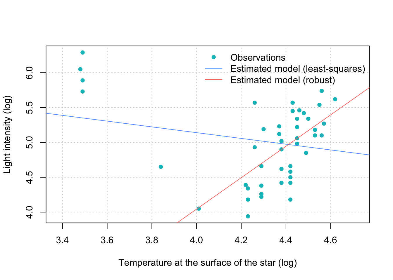
Figure B.2: Comparison of Estimation Methodologies on 47 observations from the Hertzsprung-Russell diagram of the star cluster CYG OB1 in the direction of Cygnus.
From Figure B.2 it can be seen that classical linear regression is considerably affected by the cloud of apparent outliers on the left hand side of the plot. As a result, the regression line has a negative slope when the majority of the data appears to have a clear positive linear trend. The latter is however the case when using a robust approach which indeed detects a positive linear trend. Having said this, there are in fact two distinct populations in the data consisting in “giants” (upper left corner) and “main sequencers” (right handside). Thus, when observing data in general it is always necessary to understand if we are dealing with real outliers (unexplained outlying data) or simply with data that can be explained by other factors (e.g. a different population as in this example).
summary(LS)##
## Call:
## lm(formula = starsCYG$log.light ~ starsCYG$log.Te)
##
## Residuals:
## Min 1Q Median 3Q Max
## -1.1052 -0.5067 0.1327 0.4423 0.9390
##
## Coefficients:
## Estimate Std. Error t value Pr(>|t|)
## (Intercept) 6.7935 1.2365 5.494 1.75e-06 ***
## starsCYG$log.Te -0.4133 0.2863 -1.444 0.156
## ---
## Signif. codes: 0 '***' 0.001 '**' 0.01 '*' 0.05 '.' 0.1 ' ' 1
##
## Residual standard error: 0.5646 on 45 degrees of freedom
## Multiple R-squared: 0.04427, Adjusted R-squared: 0.02304
## F-statistic: 2.085 on 1 and 45 DF, p-value: 0.1557summary(rob)##
## Call:
## lmrob(formula = starsCYG$log.light ~ starsCYG$log.Te)
## \--> method = "MM"
## Residuals:
## Min 1Q Median 3Q Max
## -0.80959 -0.28838 0.00282 0.36668 3.39585
##
## Coefficients:
## Estimate Std. Error t value Pr(>|t|)
## (Intercept) -4.9694 3.4100 -1.457 0.15198
## starsCYG$log.Te 2.2532 0.7691 2.930 0.00531 **
## ---
## Signif. codes: 0 '***' 0.001 '**' 0.01 '*' 0.05 '.' 0.1 ' ' 1
##
## Robust residual standard error: 0.4715
## Multiple R-squared: 0.3737, Adjusted R-squared: 0.3598
## Convergence in 15 IRWLS iterations
##
## Robustness weights:
## 4 observations c(11,20,30,34) are outliers with |weight| = 0 ( < 0.0021);
## 4 weights are ~= 1. The remaining 39 ones are summarized as
## Min. 1st Qu. Median Mean 3rd Qu. Max.
## 0.6533 0.9171 0.9593 0.9318 0.9848 0.9986
## Algorithmic parameters:
## tuning.chi bb tuning.psi refine.tol
## 1.548e+00 5.000e-01 4.685e+00 1.000e-07
## rel.tol scale.tol solve.tol eps.outlier
## 1.000e-07 1.000e-10 1.000e-07 2.128e-03
## eps.x warn.limit.reject warn.limit.meanrw
## 8.404e-12 5.000e-01 5.000e-01
## nResample max.it best.r.s k.fast.s k.max
## 500 50 2 1 200
## maxit.scale trace.lev mts compute.rd fast.s.large.n
## 200 0 1000 0 2000
## psi subsampling cov
## "bisquare" "nonsingular" ".vcov.avar1"
## compute.outlier.stats
## "SM"
## seed : int(0)C Proofs
Ronchetti, E.M. 2006. “The Historical Development of Robust Statistics.”
Duncan, I., and S. Guerrier. 2016. “Member Plan Choice and Migration in Response to Changes in Member Premiums after Massachusetts Health Insurance Reform.” North American Actuarial Journal.
Huber, P.J., and E.M. Ronchetti. 2009. Robust Statistics. John Wiley & Sons Inc.
Anscombe, F.J., and I. Guttman. 1960. “Rejection of Outliers.” Technometrics 2 (2). The American Society for Quality Control; The American Statistical Association: 123–47.
Hampel, F.R., E.M. Ronchetti, P.J. Rousseeuw, and W.A. Stahel. 1987. Robust Statistics: the Approach Based on Influence Functions. Wiley New York.
Hampel, F.R. 1968. “Contributions to the Theory of Robust Estimation.” PhD thesis, University of California, Berkeley.
Huber, P.J. 1973. “Robust Regression: Asymptotics, Conjectures and Monte Carlo.” The Annals of Statistics 1 (5). Institute of Mathematical Statistics: 799–821.
Hampel, F.R. 1968. “Contributions to the Theory of Robust Estimation.” PhD thesis, University of California, Berkeley.
1973. “Robust Estimation: A Condensed Partial Survey.” Probability Theory and Related Fields 27 (2). Springer: 87–104.Krasker, W.S. 1980. “Estimation in Linear Regression Models with Disparate Data Points.” Econometrica 48 (6). The Econometric Society: 1333–46.
\(M\)-estimators are obtained as the minima of sums of functions of the data.↩