In this section, we will briefly show some of the simts package functionalities. In the examples shown here, time series data may take the form of either a one-column matrix, data.frame, or numeric vector.

The following three datasets stored in simts will be used as examples.

• hydro: This time series contains the monthly precipitation from 1907 and going to 1972 for total of 781 observations taken from Hipel and McLeod (1994).
• savingrt: This dataset contains the US personal saving (after removing seasonal trends) which represent the percentage of income saved from the disposable personal income. This time series with frequency 12 starting in year 1959 and going to 2016 for a total of 691 observations.
• sales: This dataset contains the US monthly clothing retail sales in millions of dollars taken from 1992 to 2016 for a total of 302 observations.
• Nile: This time series contains the measurements of the annual flow of the river Nile at Aswan (formerly Assuan), 1871–1970, in \(10^8 m^3\) taken from Table 1 of Cobb (1978).

The code below shows how to setup a time series as a gts() object. Here, we take samples from each dataset at a rate of freq ticks per sample. By applying plot() on the result of a gts() object, we can observe a simple visualization of our data.

Hydrology

Frist, we consider the hydro dataset. The code below shows how to construct a gts object and plot the resulting time series.

# Load hydro dataset
data("hydro")

# Simulate based on data
hydro = gts(as.vector(hydro), start = 1907, freq = 12, unit_ts = "in.", 
            name_ts = "Precipitation", data_name = "Precipitation data from Hipel et al., (1994)")

# Plot hydro simulation
plot(hydro)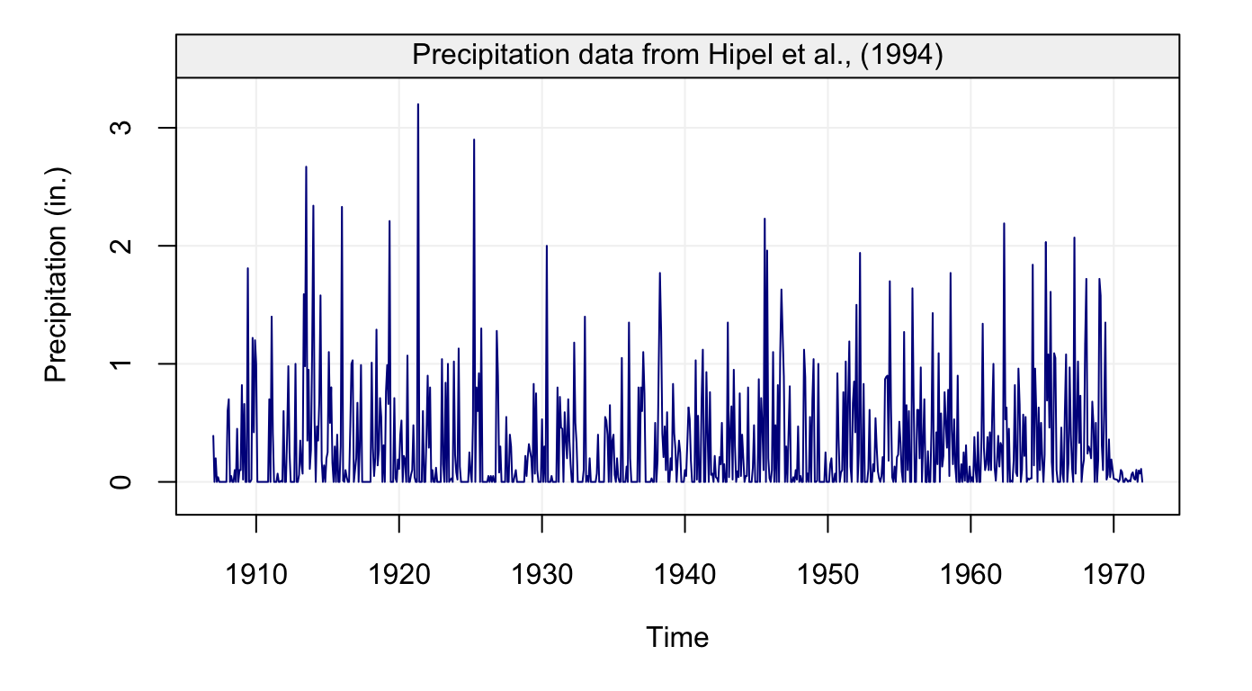

Figure 1: Monthly precipitation series from 1907 to 1972 taken from Hipel and McLeod (1994)

Using the object we created we can now compute its autocorrelation function using the ACF() function as follows:

# Compute ACF and plot result
hydro_acf = ACF(hydro)
plot(hydro_acf)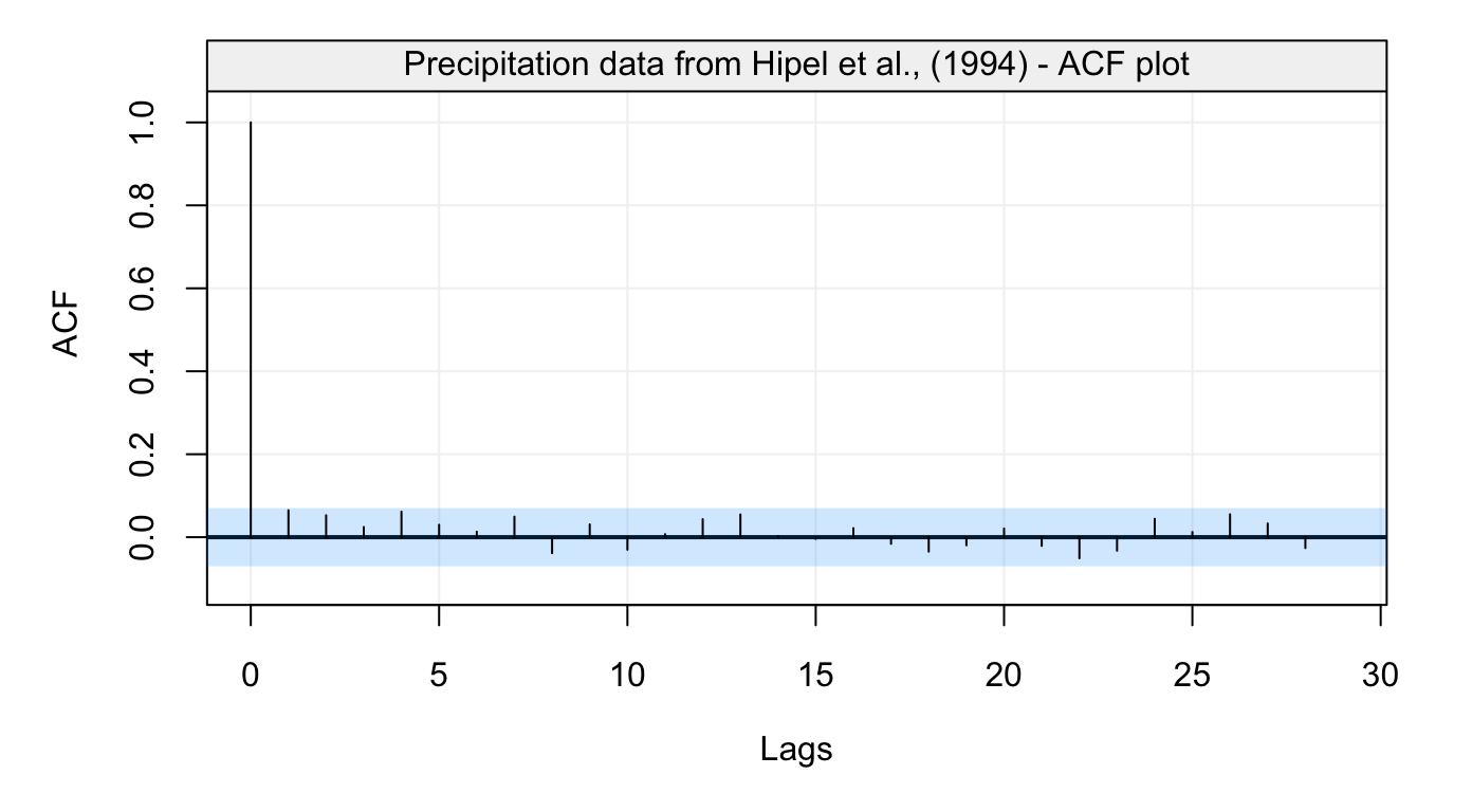

Figure 2: Empirical autocorrelation function of monthly precipitation series from Hipel and McLeod (1994)

This graph reveals that this time series does not appear to present any form of autocorrelation. A different visual analysis might be given by a robust estimator of the autocorrelation function.

Personal Savings

Similarly to the first dataset, we now consider the savingrt time series:

# Load savingrt dataset
data("savingrt")
# Simulate based on data
savingrt = gts(as.vector(savingrt), start = 1959, freq = 12, unit_ts = "%", 
            name_ts = "Saving Rates", data_name = "US Personal Saving Rates")
# Plot savingrt simulation
plot(savingrt)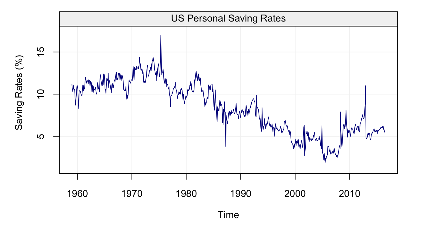

Figure 3: Monthly (seasonally adjusted) Personal Saving Rates data from January 1959 to May 2015 provided by the Federal Reserve Bank of St. Louis.

# Compute ACF and plot result
savingrt_acf = ACF(savingrt)
plot(savingrt_acf)

Figure 4: Empirical autocorrelation function of Personal Saving Rates data

This graph indicates that this time series is likely to present some non-stationary features. This is actually not a surprising observation as such data are often assumed to be close to a random walk model.

Retail Sales

Let’s consider the next dataset, the sales time series:

# Load sales dataset
data("sales")

# Simulate based on data
sales = gts(as.vector(sales), start = 1992, freq = 12, name_time = "Month",
            unit_ts = bquote(paste(10^6,"$")), name_ts = "Retail Sales", 
            data_name = "Monthly Clothing Retail Sales in US for 1992-2016")


# Plot sales simulation
plot(sales)

Figure 5: Monthly Clothing Retail Sales in US for 1992-2016

After creating the time series object, now we can compute its autocorrelation function and partial autocorrelation function by using ACF() and PACF() as follows:

# Compute ACF and plot result
sales_acf = ACF(sales)
plot(sales_acf)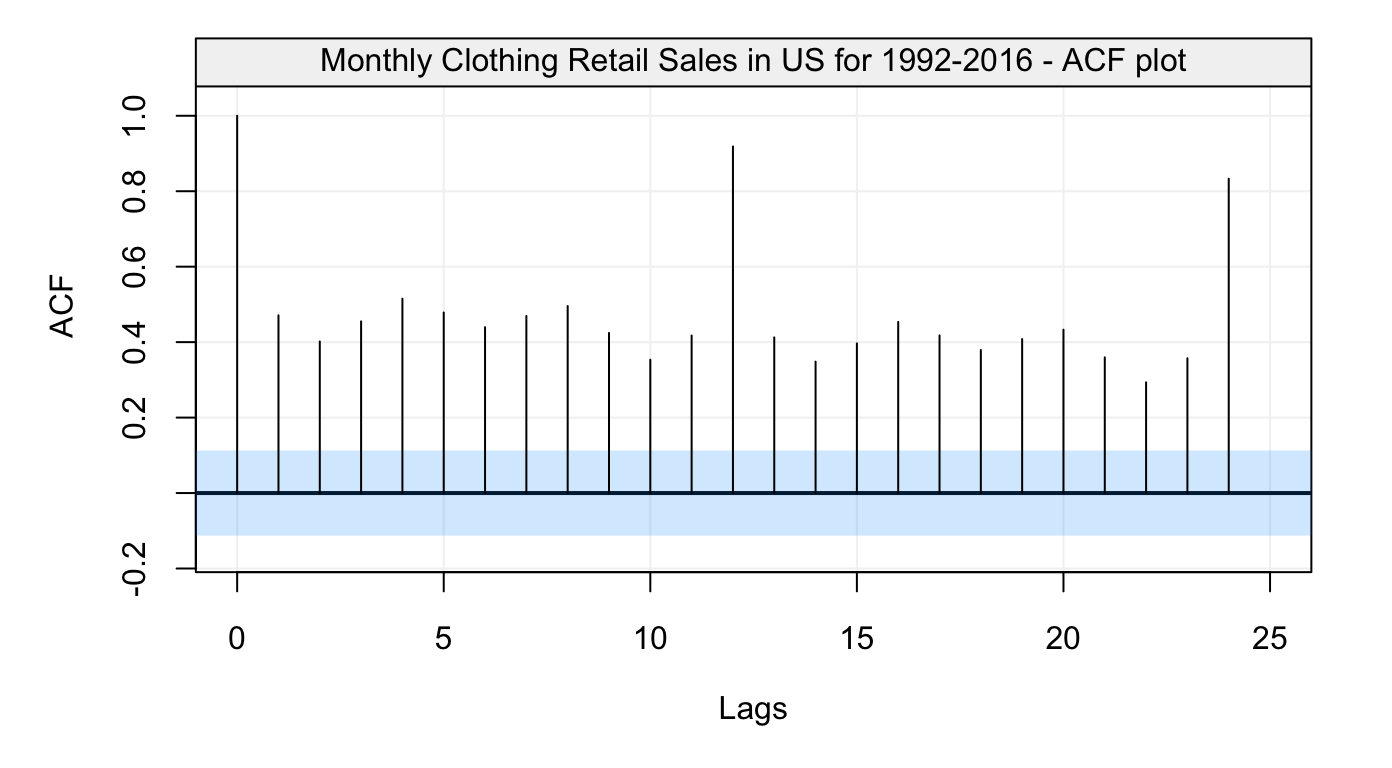

Figure 6: Empirical autocorrelation function of Monthly Clothing Retail Sales in US for 1992-2016

#Compute PACF and plot result
sales_pacf = PACF(sales)
plot(sales_pacf)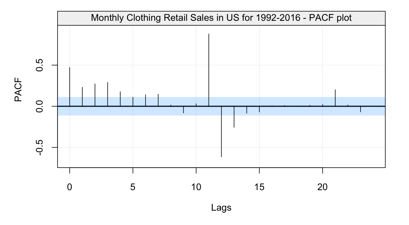

Figure 7: Empirical partial autocorrelation function of Monthly Clothing Retail Sales in US for 1992-2016

You can also use corr_analysis() function in the package to get the same results as above:

# Compute and plot ACF and PACF
sales_corr = corr_analysis(sales)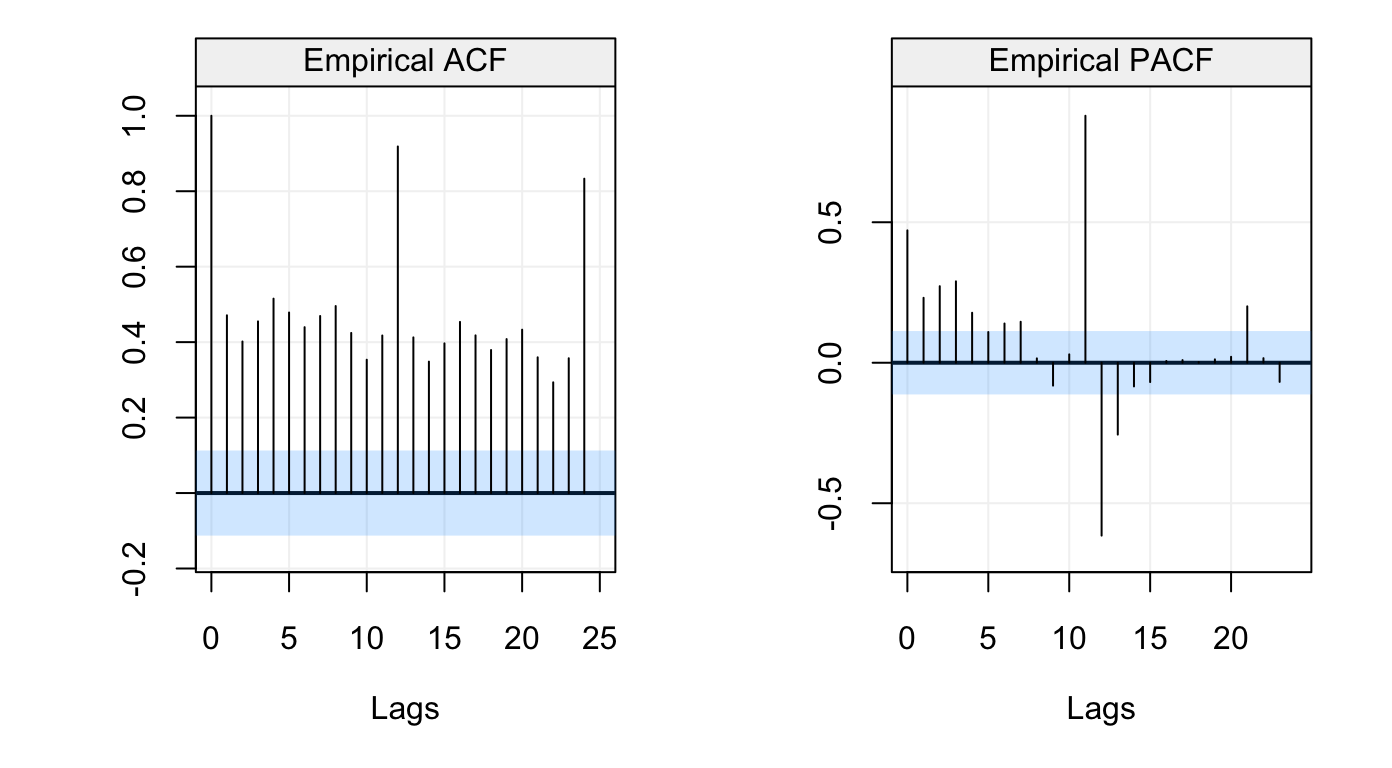

Figure 8: Empirical ACF and PACF of Monthly Clothing Retail Sales in US for 1992-2016

# Get ACF and PACF values
sales_acf = sales_corr$ACF
sales_pacf = sales_corr$PACF

The autocorrelation graph reveals that there exits some seasonal features in this time series. As we can expect, the sales data is likely to present similar behaviors from year to year.

Nile River Flow

Finally, we consider the last dataset in the code below:

# Load Nile dataset
Nile = datasets::Nile

# Simulate based on data
nile = gts(as.vector(Nile), start = 1871, end = 1970, freq = 1, 
           unit_ts = bquote(paste(10^8," ",m^3)), name_ts = "Flow", 
           name_time = "Years", data_name = "Annual Flow of the Nile River")

# Plot Nile simulation 
plot(nile)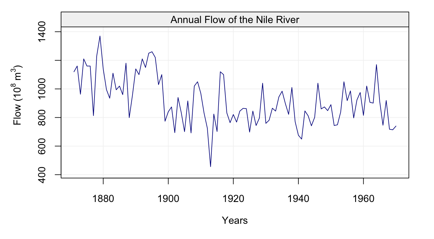

Figure 9: Plot of Annual Nile river flow from 1871-1970

To get ACF, we can use ACF() and make a plot:

# Compute ACF and plot result
nile_acf = ACF(nile)
plot(nile_acf)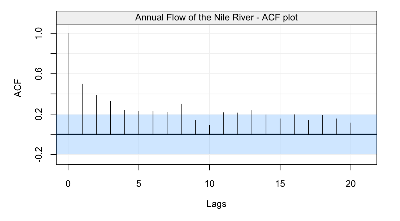

Figure 10: Empirical autocorrelation function of the Nile river flow data

Similar to the example above, we can also use corr_analysis() to get the ACF and PACF at the same time:

# Compute and plot ACF and PACF
nile_corr = corr_analysis(nile)

Figure 11: Empirical ACF and PACF of the Nile river flow data

# Get ACF and PACF values
nile_acf = nile_corr$ACF
nile_pacf = nile_corr$PACF

Missing features:

• Add new dataset
• Add robust estimators
• Add content of “Sample Analyses using exts” to the packages and the appropriate vignettes
• Add content (similarly to above) of “Experimental Time Series Features”
• Check slides and add content to this page (see forecast function)

References

Cobb, George W. 1978. “The Problem of the Nile: Conditional Solution to a Changepoint Problem.” Biometrika. JSTOR, 243–51.

Hipel, Keith W, and A Ian McLeod. 1994. Time Series Modelling of Water Resources and Environmental Systems. Vol. 45. Elsevier.