plot multiple nees.stat objects alltogether
Usage
# S3 method for class 'nees.stat'
plot(..., alpha = 0.95, legend = NA, title = NA)Value
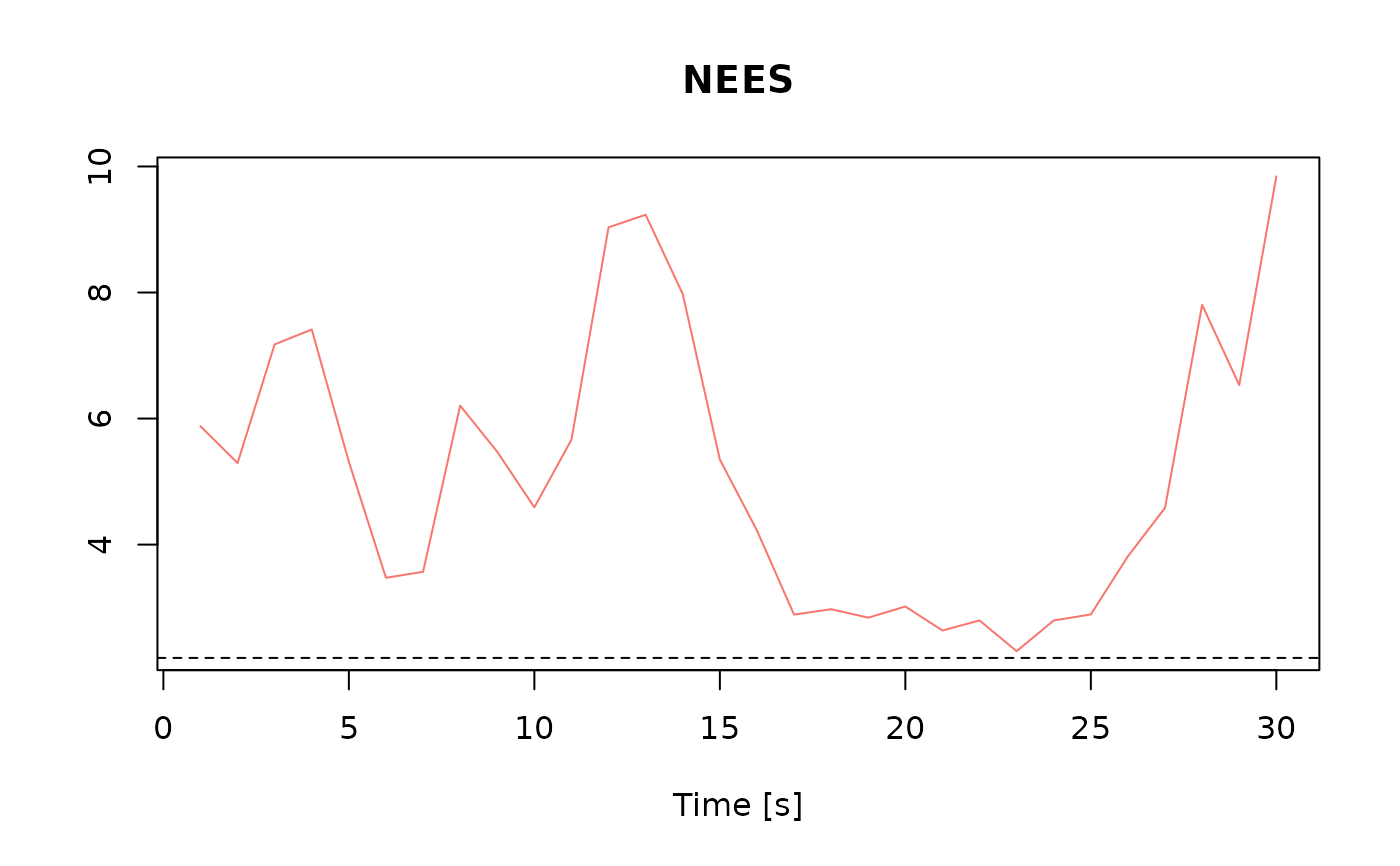
Produce a plot of the Normalized Estimation Error Squared (NEES) for the nees.stat object provided.
Examples
data("lemniscate_traj_ned")
head(lemniscate_traj_ned)
#> t x y z roll pitch_sm yaw
#> [1,] 0.00 0.00000000 0.00000000 0 0.0000000000 0.000000e+00 0.7853979
#> [2,] 0.01 0.05235987 0.05235984 0 0.0001821107 8.255405e-05 0.7853971
#> [3,] 0.02 0.10471968 0.10471945 0 0.0003642249 1.650525e-04 0.7853946
#> [4,] 0.03 0.15707937 0.15707860 0 0.0005463461 2.474976e-04 0.7853905
#> [5,] 0.04 0.20943890 0.20943706 0 0.0007284778 3.298918e-04 0.7853847
#> [6,] 0.05 0.26179819 0.26179460 0 0.0009106235 4.122374e-04 0.7853773
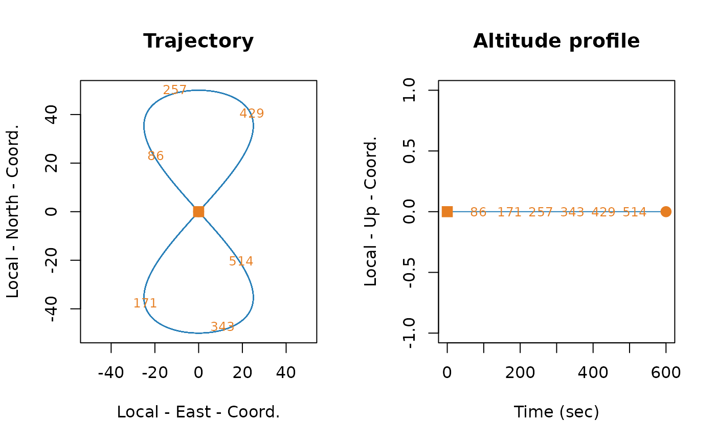
traj <- make_trajectory(data = lemniscate_traj_ned, system = "ned")
plot(traj)
 timing <- make_timing(
nav.start = 0, # time at which to begin filtering
nav.end = 30,
freq.imu = 100, # frequency of the IMU, can be slower wrt trajectory frequency
freq.gps = 1, # GNSS frequency
freq.baro = 1, # barometer frequency (to disable, put it very low, e.g. 1e-5)
gps.out.start = 20, # to simulate a GNSS outage, set a time before nav.end
gps.out.end = 25
)
# create sensor for noise data generation
snsr.mdl <- list()
# this uses a model for noise data generation
acc.mdl <- WN(sigma2 = 5.989778e-05) +
AR1(phi = 9.982454e-01, sigma2 = 1.848297e-10) +
AR1(phi = 9.999121e-01, sigma2 = 2.435414e-11) +
AR1(phi = 9.999998e-01, sigma2 = 1.026718e-12)
gyr.mdl <- WN(sigma2 = 1.503793e-06) +
AR1(phi = 9.968999e-01, sigma2 = 2.428980e-11) +
AR1(phi = 9.999001e-01, sigma2 = 1.238142e-12)
snsr.mdl$imu <- make_sensor(
name = "imu",
frequency = timing$freq.imu,
error_model1 = acc.mdl,
error_model2 = gyr.mdl
)
# RTK-like GNSS
gps.mdl.pos.hor <- WN(sigma2 = 0.025^2)
gps.mdl.pos.ver <- WN(sigma2 = 0.05^2)
gps.mdl.vel.hor <- WN(sigma2 = 0.01^2)
gps.mdl.vel.ver <- WN(sigma2 = 0.02^2)
snsr.mdl$gps <- make_sensor(
name = "gps",
frequency = timing$freq.gps,
error_model1 = gps.mdl.pos.hor,
error_model2 = gps.mdl.pos.ver,
error_model3 = gps.mdl.vel.hor,
error_model4 = gps.mdl.vel.ver
)
# Barometer
baro.mdl <- WN(sigma2 = 0.5^2)
snsr.mdl$baro <- make_sensor(
name = "baro",
frequency = timing$freq.baro,
error_model1 = baro.mdl
)
# define sensor for Kalmna filter
KF.mdl <- list()
# make IMU sensor
KF.mdl$imu <- make_sensor(
name = "imu",
frequency = timing$freq.imu,
error_model1 = acc.mdl,
error_model2 = gyr.mdl
)
KF.mdl$gps <- snsr.mdl$gps
KF.mdl$baro <- snsr.mdl$baro
# perform navigation simulation
num.runs <- 2 # number of Monte-Carlo simulations
res <- navigation(
traj.ref = traj,
timing = timing,
snsr.mdl = snsr.mdl,
KF.mdl = KF.mdl,
num.runs = num.runs,
noProgressBar = TRUE,
PhiQ_method = "1",
# order of the Taylor expansion of the matrix exponential used to compute Phi and Q matrices
compute_PhiQ_each_n = 10,
# compute new Phi and Q matrices every n IMU steps (execution time optimization)
parallel.ncores = 1,
P_subsampling = timing$freq.imu
)
nees <- compute_nees(res, idx = 1:6, step = 100)
#>
#>
plot(nees)
timing <- make_timing(
nav.start = 0, # time at which to begin filtering
nav.end = 30,
freq.imu = 100, # frequency of the IMU, can be slower wrt trajectory frequency
freq.gps = 1, # GNSS frequency
freq.baro = 1, # barometer frequency (to disable, put it very low, e.g. 1e-5)
gps.out.start = 20, # to simulate a GNSS outage, set a time before nav.end
gps.out.end = 25
)
# create sensor for noise data generation
snsr.mdl <- list()
# this uses a model for noise data generation
acc.mdl <- WN(sigma2 = 5.989778e-05) +
AR1(phi = 9.982454e-01, sigma2 = 1.848297e-10) +
AR1(phi = 9.999121e-01, sigma2 = 2.435414e-11) +
AR1(phi = 9.999998e-01, sigma2 = 1.026718e-12)
gyr.mdl <- WN(sigma2 = 1.503793e-06) +
AR1(phi = 9.968999e-01, sigma2 = 2.428980e-11) +
AR1(phi = 9.999001e-01, sigma2 = 1.238142e-12)
snsr.mdl$imu <- make_sensor(
name = "imu",
frequency = timing$freq.imu,
error_model1 = acc.mdl,
error_model2 = gyr.mdl
)
# RTK-like GNSS
gps.mdl.pos.hor <- WN(sigma2 = 0.025^2)
gps.mdl.pos.ver <- WN(sigma2 = 0.05^2)
gps.mdl.vel.hor <- WN(sigma2 = 0.01^2)
gps.mdl.vel.ver <- WN(sigma2 = 0.02^2)
snsr.mdl$gps <- make_sensor(
name = "gps",
frequency = timing$freq.gps,
error_model1 = gps.mdl.pos.hor,
error_model2 = gps.mdl.pos.ver,
error_model3 = gps.mdl.vel.hor,
error_model4 = gps.mdl.vel.ver
)
# Barometer
baro.mdl <- WN(sigma2 = 0.5^2)
snsr.mdl$baro <- make_sensor(
name = "baro",
frequency = timing$freq.baro,
error_model1 = baro.mdl
)
# define sensor for Kalmna filter
KF.mdl <- list()
# make IMU sensor
KF.mdl$imu <- make_sensor(
name = "imu",
frequency = timing$freq.imu,
error_model1 = acc.mdl,
error_model2 = gyr.mdl
)
KF.mdl$gps <- snsr.mdl$gps
KF.mdl$baro <- snsr.mdl$baro
# perform navigation simulation
num.runs <- 2 # number of Monte-Carlo simulations
res <- navigation(
traj.ref = traj,
timing = timing,
snsr.mdl = snsr.mdl,
KF.mdl = KF.mdl,
num.runs = num.runs,
noProgressBar = TRUE,
PhiQ_method = "1",
# order of the Taylor expansion of the matrix exponential used to compute Phi and Q matrices
compute_PhiQ_each_n = 10,
# compute new Phi and Q matrices every n IMU steps (execution time optimization)
parallel.ncores = 1,
P_subsampling = timing$freq.imu
)
nees <- compute_nees(res, idx = 1:6, step = 100)
#>
#>
plot(nees)