First of all, we need to load the reference trajectory and create a
trajectory object out of it (see
?make_trajectory for details).
##         t          x          y z         roll     pitch_sm       yaw
## [1,] 0.00 0.00000000 0.00000000 0 0.0000000000 0.000000e+00 0.7853979
## [2,] 0.01 0.05235987 0.05235984 0 0.0001821107 8.255405e-05 0.7853971
## [3,] 0.02 0.10471968 0.10471945 0 0.0003642249 1.650525e-04 0.7853946
## [4,] 0.03 0.15707937 0.15707860 0 0.0005463461 2.474976e-04 0.7853905
## [5,] 0.04 0.20943890 0.20943706 0 0.0007284778 3.298918e-04 0.7853847
## [6,] 0.05 0.26179819 0.26179460 0 0.0009106235 4.122374e-04 0.7853773
traj <- make_trajectory(data = lemniscate_traj_ned, system = "ned")Let’s see how the reference trajectory looks like.
# plot traj
plot(traj, n_split = 6)
plot(traj, threeD = TRUE)Then we need to make a timing object (see
?make_timing for details) where we specify
- the start and the end of navigation,
- the frequencies of different sensors,
- the beginning and end of the GPS outage period.
timing <- make_timing(
  nav.start = 0, # time at which to begin filtering
  nav.end = 100,
  freq.imu = 100, # frequency of the IMU, can be slower wrt trajectory frequency
  freq.gps = 1, # GNSS frequency
  freq.baro = 1, # barometer frequency (to disable, put it very low, e.g. 1e-5)
  gps.out.start = 60 , # to simulate a GNSS outage, set a time before nav.end
  gps.out.end = 80
)
Now we need to create the sensor error models for error generation as
a list of sensor objects (see ?make_sensor for
details). These are the models that will be used in generating the
sensor errors, and not the ones necessarily used within the navigation
filter.
snsr.mdl <- list()

# this uses a model for noise data generation
acc.mdl <- WN(sigma2 = 5.989778e-05) + AR1(phi = 9.982454e-01, sigma2 = 1.848297e-10) + AR1(phi = 9.999121e-01, sigma2 = 2.435414e-11) + AR1(phi = 9.999998e-01, sigma2 = 1.026718e-12)

gyr.mdl <- WN(sigma2 = 1.503793e-06) + AR1(phi = 9.968999e-01, sigma2 = 2.428980e-11) + AR1(phi = 9.999001e-01, sigma2 = 1.238142e-12)
snsr.mdl$imu <- make_sensor(name = "imu", frequency = timing$freq.imu, error_model1 = acc.mdl, error_model2 = gyr.mdl)

# RTK-like GNSS
gps.mdl.pos.hor <- WN(sigma2 = 0.025^2)
gps.mdl.pos.ver <- WN(sigma2 = 0.05^2)
gps.mdl.vel.hor <- WN(sigma2 = 0.01^2)
gps.mdl.vel.ver <- WN(sigma2 = 0.02^2)
snsr.mdl$gps <- make_sensor(
  name = "gps",
  frequency = timing$freq.gps,
  error_model1 = gps.mdl.pos.hor,
  error_model2 = gps.mdl.pos.ver,
  error_model3 = gps.mdl.vel.hor,
  error_model4 = gps.mdl.vel.ver
)

# Barometer
baro.mdl <- WN(sigma2 = 0.5^2)
snsr.mdl$baro <- make_sensor(name = "baro", frequency = timing$freq.baro, error_model1 = baro.mdl)
Then we need to create the sensor error models for filtering as a
list of sensor objects (see ?make_sensor for
details). These are the models that will be used within the navigation
filter (an extended Kalman filter), which may or may not be the same as
the ones used in generating the sensor errors. In this example, we have
chosen them to be the same.
KF.mdl <- list()

# make IMU sensor
KF.mdl$imu <- make_sensor(name = "imu", frequency = timing$freq.imu, error_model1 = acc.mdl, error_model2 = gyr.mdl)

KF.mdl$gps <- snsr.mdl$gps
KF.mdl$baro <- snsr.mdl$baro
Finally, we can call the navigation function, which
first simulates realistic sensor data based on the reference trajectory
and provided sensor error models, and then performs the navigation. The
whole process can be done in a Monte-Carlo fashion, by only specifying
the number of desired runs as the num.runs input to
navigation function. For detailed documentation, see
?navigation.
num.runs <- 20 # number of Monte-Carlo simulations
res <- navigation(
  traj.ref = traj,
  timing = timing,
  snsr.mdl = snsr.mdl,
  KF.mdl = KF.mdl,
  num.runs = num.runs,
  noProgressBar = TRUE,
  PhiQ_method = "1", # order of the Taylor expansion of the matrix exponential used to compute Phi and Q matrices
  compute_PhiQ_each_n = 20, # compute new Phi and Q matrices every n IMU steps (execution time optimization)
  parallel.ncores = 1,
  P_subsampling = timing$freq.imu
) # keep one covariance every second
We can now see how the results look like.
plot(res, plot3d = F, error_analysis = T)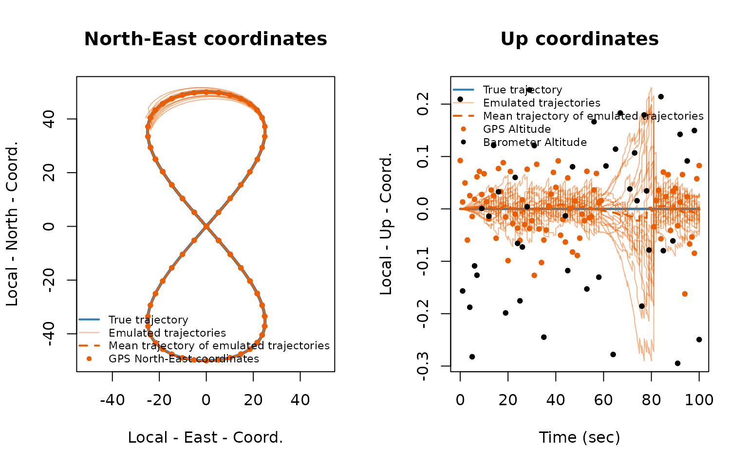

We can now compute statistics of the navigation performance based on the Monte Carlo simulation.
# mean position error
pe <- compute_mean_position_err(res, step = 25)

# mean orientation error
oe <- compute_mean_orientation_err(res, step = 25)
# NEES
nees <- compute_nees(res, idx = 1:6, step = 100)

# Empirical coverage
coverage <- compute_coverage(res, alpha = 0.7, step = 100, idx = 1:6)
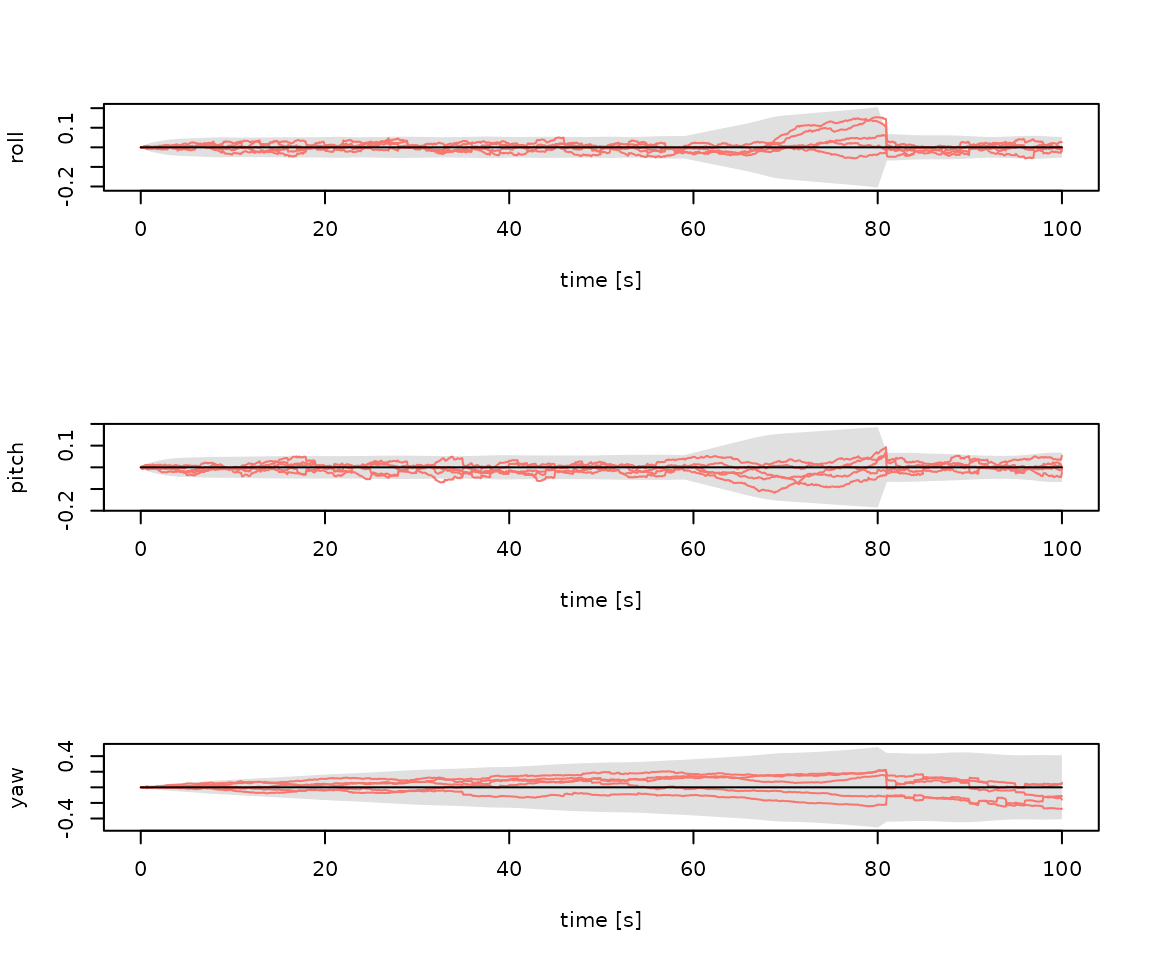
We can plot the computed statistics
plot_imu_err_with_cov(res, error = FALSE)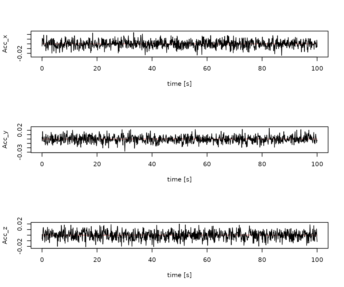
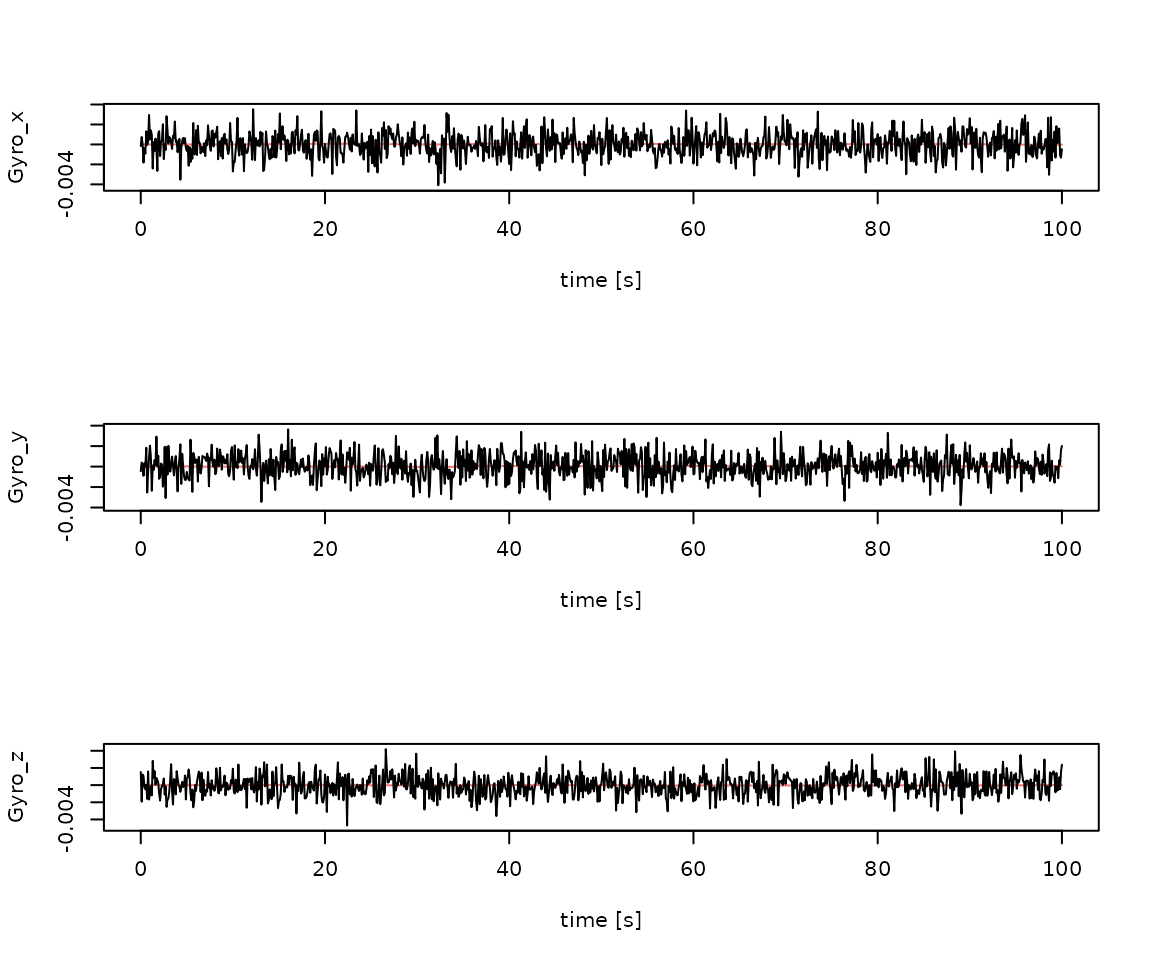
plot_nav_states_with_cov(res, idx = 1:5, error = TRUE)
plot(pe)
plot(oe)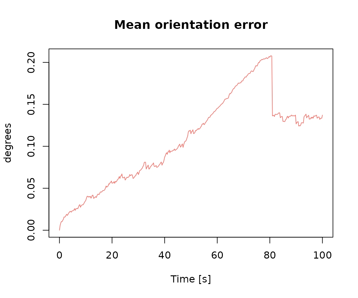
plot(nees)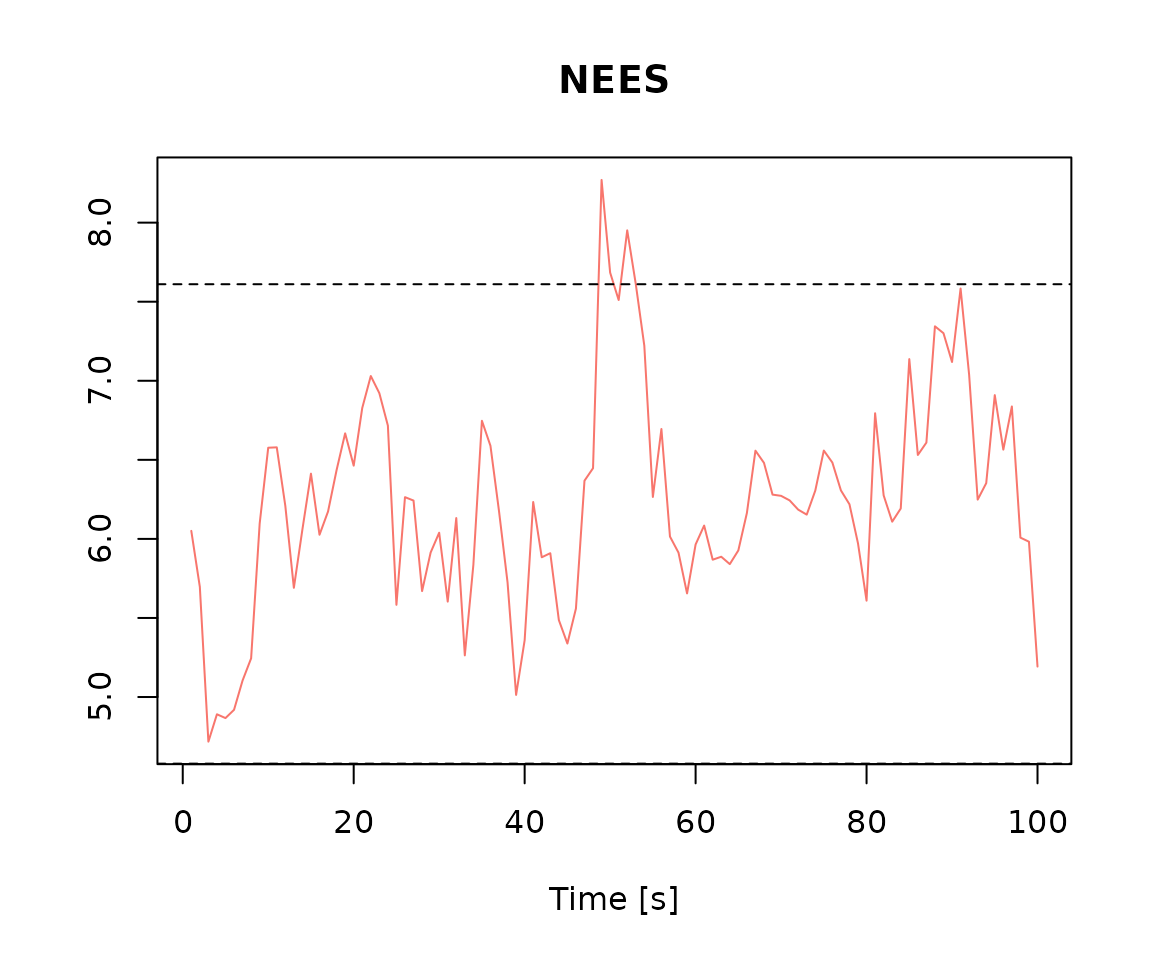
plot(coverage)