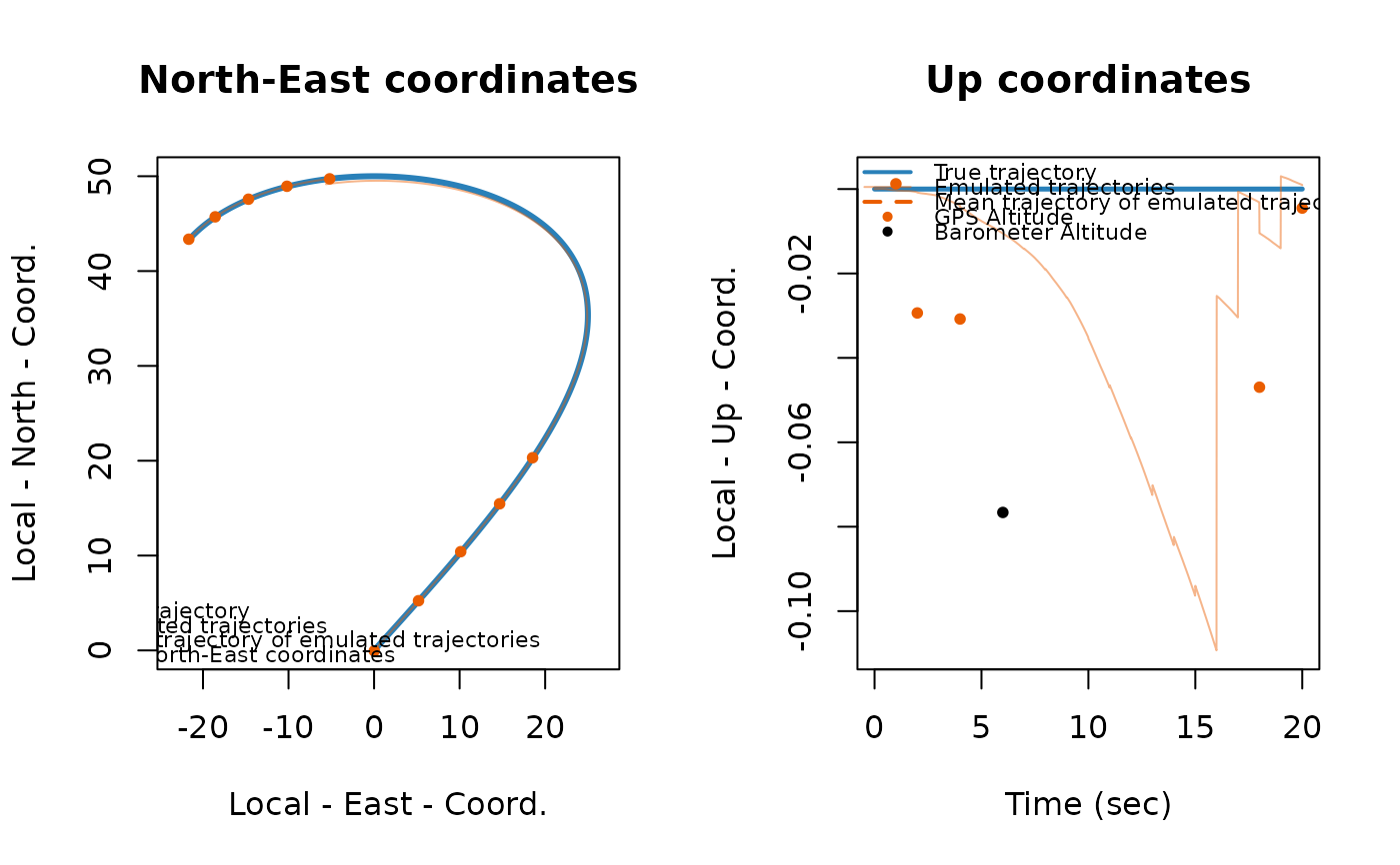
This function enables the visualization of a navigation object, both in 2d and in 3d. The function therefore enables
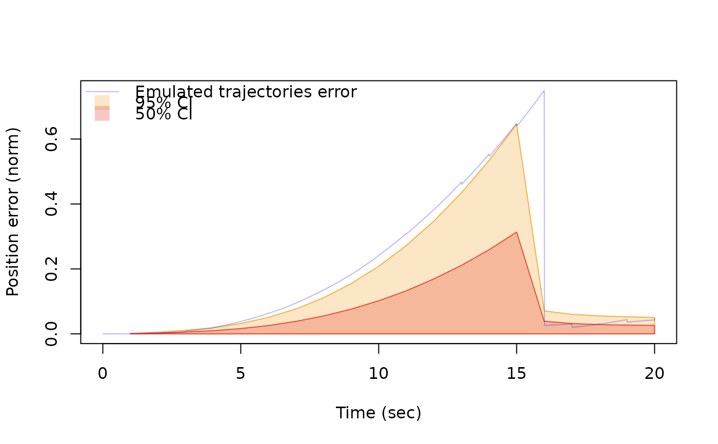
the comparison of the true trajectory with emulated trajectories. One can also plot the analysis of the error of the trajectories
by comparing the L2 norm of the difference between emulated trajectories and the true trajectory over time.
Usage
# S3 method for class 'navigation'
plot(
  x,
  true_col = "#2980b9",
  col_fused_trans = "#EA5D0073",
  col_fused_full = "#EA5D00FF",
  plot_mean_traj = TRUE,
  plot_baro = TRUE,
  baro_col = "black",
  emu_to_plot = 1,
  plot3d = FALSE,
  plot_CI = FALSE,
  time_interval = 5,
  col_50 = "#E74C3C4D",
  col_95 = "#F5B0414D",
  col_50_brd = "#E74C3C",
  col_95_brd = "#F5B041",
  error_analysis = FALSE,
  emu_for_covmat = 1,
  nsim = 1000,
  col_traj_error = "#1C12F54D",
  time_interval_simu = 0.5,
  seed = 123,
  ...
)
Arguments
- x
A
navigationobject- true_col
The color of the true trajectory
- col_fused_trans
The color of the emulated trajectories
- col_fused_full
The color of the mean trajectory of the emulated trajectories
- plot_mean_traj
A Boolean indicating whether or not to plot the mean mean trajectory of the emulated trajectories. Default is
True- plot_baro
A Boolean indicating whether or not to plot the barometer datapoint in tha Up coordinates plot. Default is
True- baro_col
The color of the barometer datapoints
- emu_to_plot
The emulated trajectory for which to plot confidence ellipses on the North-East coordinates plot
- plot3d
A Boolean indicating whether or not to plot the 3d plot of the trajectory
- plot_CI
A Boolean indicating whether or not to plot the confidence intervals for both 2d plots
- time_interval
A value in seconds indicating the interval at which to plot the CI on the North-East coordinates plot
- col_50
The color for the 50% confidence intervals.
- col_95
The color for the 95% confidence intervals.
- col_50_brd
The color for the 50% confidence intervals borders.
- col_95_brd
The color for the 95% confidence intervals.
- error_analysis
A Boolean indicating whether or not to display an error analysis plot of the emulated trajectories
- emu_for_covmat
The emulated trajectory for which to use the var-cov matrix in order to simulate data and compute the CI of the error
- nsim
An integer indicating the number of trajectories simulated in order to compute the CI
- col_traj_error
The color for the trajectory estimation error
- time_interval_simu
time interval simu
- seed
A seed for plotting
- ...
additional plotting argument
Examples
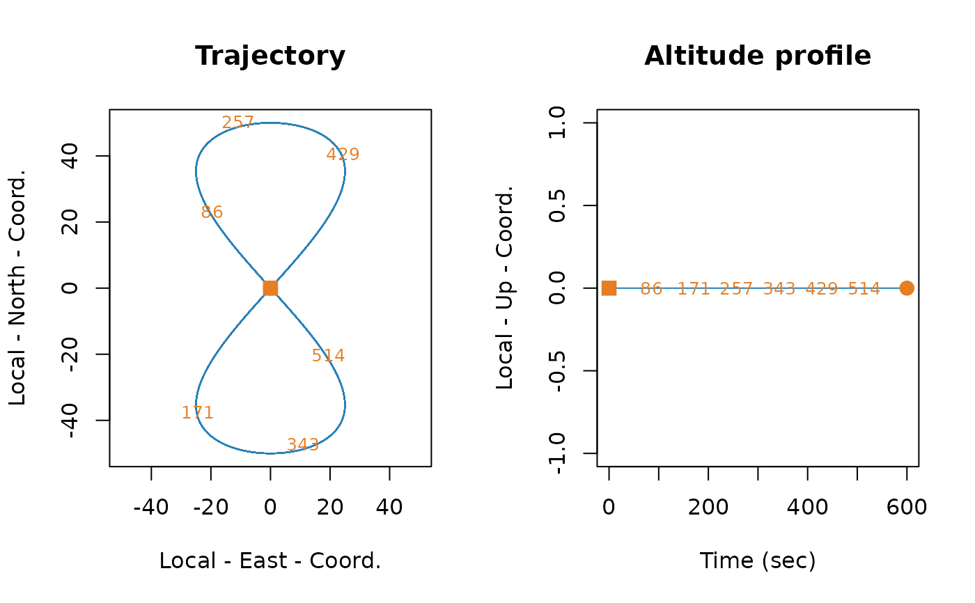
data("lemniscate_traj_ned")
head(lemniscate_traj_ned)
#> t x y z roll pitch_sm yaw
#> [1,] 0.00 0.00000000 0.00000000 0 0.0000000000 0.000000e+00 0.7853979
#> [2,] 0.01 0.05235987 0.05235984 0 0.0001821107 8.255405e-05 0.7853971
#> [3,] 0.02 0.10471968 0.10471945 0 0.0003642249 1.650525e-04 0.7853946
#> [4,] 0.03 0.15707937 0.15707860 0 0.0005463461 2.474976e-04 0.7853905
#> [5,] 0.04 0.20943890 0.20943706 0 0.0007284778 3.298918e-04 0.7853847
#> [6,] 0.05 0.26179819 0.26179460 0 0.0009106235 4.122374e-04 0.7853773
traj <- make_trajectory(data = lemniscate_traj_ned, system = "ned")
plot(traj)
 timing <- make_timing(
nav.start = 0, # time at which to begin filtering
nav.end = 20,
freq.imu = 100, # frequency of the IMU, can be slower wrt trajectory frequency
freq.gps = 1, # GNSS frequency
freq.baro = 1, # barometer frequency (to disable, put it very low, e.g. 1e-5)
gps.out.start = 5, # to simulate a GNSS outage, set a time before nav.end
gps.out.end = 15
)
# create sensor for noise data generation
snsr.mdl <- list()
# this uses a model for noise data generation
acc.mdl <- WN(sigma2 = 5.989778e-05) +
AR1(phi = 9.982454e-01, sigma2 = 1.848297e-10) +
AR1(phi = 9.999121e-01, sigma2 = 2.435414e-11) +
AR1(phi = 9.999998e-01, sigma2 = 1.026718e-12)
gyr.mdl <- WN(sigma2 = 1.503793e-06) +
AR1(phi = 9.968999e-01, sigma2 = 2.428980e-11) +
AR1(phi = 9.999001e-01, sigma2 = 1.238142e-12)
snsr.mdl$imu <- make_sensor(
name = "imu",
frequency = timing$freq.imu,
error_model1 = acc.mdl,
error_model2 = gyr.mdl
)
# RTK-like GNSS
gps.mdl.pos.hor <- WN(sigma2 = 0.025^2)
gps.mdl.pos.ver <- WN(sigma2 = 0.05^2)
gps.mdl.vel.hor <- WN(sigma2 = 0.01^2)
gps.mdl.vel.ver <- WN(sigma2 = 0.02^2)
snsr.mdl$gps <- make_sensor(
name = "gps",
frequency = timing$freq.gps,
error_model1 = gps.mdl.pos.hor,
error_model2 = gps.mdl.pos.ver,
error_model3 = gps.mdl.vel.hor,
error_model4 = gps.mdl.vel.ver
)
# Barometer
baro.mdl <- WN(sigma2 = 0.5^2)
snsr.mdl$baro <- make_sensor(
name = "baro",
frequency = timing$freq.baro,
error_model1 = baro.mdl
)
# define sensor for Kalmna filter
KF.mdl <- list()
# make IMU sensor
KF.mdl$imu <- make_sensor(
name = "imu",
frequency = timing$freq.imu,
error_model1 = acc.mdl,
error_model2 = gyr.mdl
)
KF.mdl$gps <- snsr.mdl$gps
KF.mdl$baro <- snsr.mdl$baro
# perform navigation simulation
num.runs <- 1 # number of Monte-Carlo simulations
res <- navigation(
traj.ref = traj,
timing = timing,
snsr.mdl = snsr.mdl,
KF.mdl = KF.mdl,
num.runs = num.runs,
noProgressBar = TRUE,
PhiQ_method = "3",
# order of the Taylor expansion of the matrix exponential used to compute Phi and Q matrices
compute_PhiQ_each_n = 10,
# compute new Phi and Q matrices every n IMU steps (execution time optimization)
parallel.ncores = 1,
P_subsampling = timing$freq.imu
)
plot(res)
timing <- make_timing(
nav.start = 0, # time at which to begin filtering
nav.end = 20,
freq.imu = 100, # frequency of the IMU, can be slower wrt trajectory frequency
freq.gps = 1, # GNSS frequency
freq.baro = 1, # barometer frequency (to disable, put it very low, e.g. 1e-5)
gps.out.start = 5, # to simulate a GNSS outage, set a time before nav.end
gps.out.end = 15
)
# create sensor for noise data generation
snsr.mdl <- list()
# this uses a model for noise data generation
acc.mdl <- WN(sigma2 = 5.989778e-05) +
AR1(phi = 9.982454e-01, sigma2 = 1.848297e-10) +
AR1(phi = 9.999121e-01, sigma2 = 2.435414e-11) +
AR1(phi = 9.999998e-01, sigma2 = 1.026718e-12)
gyr.mdl <- WN(sigma2 = 1.503793e-06) +
AR1(phi = 9.968999e-01, sigma2 = 2.428980e-11) +
AR1(phi = 9.999001e-01, sigma2 = 1.238142e-12)
snsr.mdl$imu <- make_sensor(
name = "imu",
frequency = timing$freq.imu,
error_model1 = acc.mdl,
error_model2 = gyr.mdl
)
# RTK-like GNSS
gps.mdl.pos.hor <- WN(sigma2 = 0.025^2)
gps.mdl.pos.ver <- WN(sigma2 = 0.05^2)
gps.mdl.vel.hor <- WN(sigma2 = 0.01^2)
gps.mdl.vel.ver <- WN(sigma2 = 0.02^2)
snsr.mdl$gps <- make_sensor(
name = "gps",
frequency = timing$freq.gps,
error_model1 = gps.mdl.pos.hor,
error_model2 = gps.mdl.pos.ver,
error_model3 = gps.mdl.vel.hor,
error_model4 = gps.mdl.vel.ver
)
# Barometer
baro.mdl <- WN(sigma2 = 0.5^2)
snsr.mdl$baro <- make_sensor(
name = "baro",
frequency = timing$freq.baro,
error_model1 = baro.mdl
)
# define sensor for Kalmna filter
KF.mdl <- list()
# make IMU sensor
KF.mdl$imu <- make_sensor(
name = "imu",
frequency = timing$freq.imu,
error_model1 = acc.mdl,
error_model2 = gyr.mdl
)
KF.mdl$gps <- snsr.mdl$gps
KF.mdl$baro <- snsr.mdl$baro
# perform navigation simulation
num.runs <- 1 # number of Monte-Carlo simulations
res <- navigation(
traj.ref = traj,
timing = timing,
snsr.mdl = snsr.mdl,
KF.mdl = KF.mdl,
num.runs = num.runs,
noProgressBar = TRUE,
PhiQ_method = "3",
# order of the Taylor expansion of the matrix exponential used to compute Phi and Q matrices
compute_PhiQ_each_n = 10,
# compute new Phi and Q matrices every n IMU steps (execution time optimization)
parallel.ncores = 1,
P_subsampling = timing$freq.imu
)
plot(res)
 # 3D plot
plot(res, plot3d = TRUE)
plot(res, error_analysis = TRUE)
# 3D plot
plot(res, plot3d = TRUE)
plot(res, error_analysis = TRUE)