summary.swaglm
summary.swaglm.Rdsummary.swaglm
# S3 method for class 'swaglm'
summary(object, ...)Value
A list of class summary_swaglm with five elements:
- mat_selected_model
A matrix where each row represents a selected model. Columns give the indices of the variables included in that model. Models are padded with
NAto match the largest model size.- mat_beta_selected_model
A matrix containing the estimated regression coefficients (including intercept) of the selected models, stacked across all dimensions. Only models with AIC less than or equal to the lowest median AIC across all dimensions are included. Each row corresponds to a model, columns correspond to the coefficients. Rows are padded with
NAto match the largest model size.- mat_p_value_selected_model
A matrix containing the p-values associated with the estimated regression coefficients in
beta_selected_model, stacked in the same order. Each row corresponds to a model, columns correspond to the coefficients. Rows are padded withNAto match the largest model size.- vec_aic_selected_model
A numeric vector containing the AIC values of all models in
mat_selected_model, stacked across dimensions. These are the AIC values for the selected models that passed the threshold described above.- lst_estimated_beta_per_variable
A named list where each element corresponds to a variable (named
V<index>). Each element is a numeric vector containing all estimated beta coefficients for that variable across all selected models in which it appears. This summarizes the distribution of effects for each variable across the selected models.- lst_p_value_per_variable
A named list where each element corresponds to a variable (named
V<index>). Each element is a numeric vector containing all estimated p-values for that variable across all selected models in which it appears.
Model selection criterion: For each model dimension (number of variables in the model), the median AIC across all models of that dimension is computed. The smallest median AIC across all dimensions is identified. Then, all models with AIC less than or equal to this value are selected. This ensures that only relatively well-performing models across all dimensions are retained for summarization.
Examples
set.seed(12345)
n <- 2000
p <- 100
# create design matrix and vector of coefficients
Sigma <- diag(rep(1/p, p))
X <- MASS::mvrnorm(n = n, mu = rep(0, p), Sigma = Sigma)
beta = c(-15,-10,5,10,15, rep(0,p-5))
# --------------------- generate from logistic regression with an intercept of one
z <- 1 + X%*%beta
pr <- 1/(1 + exp(-z))
y <- as.factor(rbinom(n, 1, pr))
y = as.numeric(y)-1
# define swag parameters
quantile_alpha = .15
p_max = 20
swaglm_obj = swaglm::swaglm(X=X, y = y, p_max = p_max, family = stats::binomial(),
alpha = quantile_alpha, verbose = TRUE, seed = 123)
#> Completed models of dimension 1
#> Completed models of dimension 2
#> Completed models of dimension 3
#> Completed models of dimension 4
#> Completed models of dimension 5
#> Completed models of dimension 6
#> Completed models of dimension 7
#> Completed models of dimension 8
#> Completed models of dimension 9
#> Completed models of dimension 10
#> Completed models of dimension 11
#> Completed models of dimension 12
#> Completed models of dimension 13
#> Completed models of dimension 14
#> Completed models of dimension 15
swaglm_obj
#> SWAGLM results :
#> -----------------------------------------
#> Input matrix dimension: 2000 100
#> Number of explored models: 863
#> Number of dimensions explored: 15
swaglm_summ = summary(swaglm_obj)
swaglm_summ$mat_selected_model
#> [,1] [,2] [,3] [,4] [,5] [,6] [,7] [,8] [,9] [,10] [,11]
#> [1,] 1 2 3 4 5 8 16 86 NA NA NA
#> [2,] 1 2 3 4 5 8 16 50 86 NA NA
#> [3,] 1 2 3 4 5 8 16 63 86 NA NA
#> [4,] 1 2 3 4 5 8 16 35 86 NA NA
#> [5,] 1 2 3 4 5 8 16 86 95 NA NA
#> [6,] 1 2 3 4 5 8 16 34 86 NA NA
#> [7,] 1 2 3 4 5 8 16 51 86 NA NA
#> [8,] 1 2 3 4 5 8 16 77 86 NA NA
#> [9,] 1 2 3 4 5 8 16 34 50 86 NA
#> [10,] 1 2 3 4 5 8 16 34 63 86 NA
#> [11,] 1 2 3 4 5 8 16 35 50 86 NA
#> [12,] 1 2 3 4 5 8 16 35 63 86 NA
#> [13,] 1 2 3 4 5 8 16 50 63 86 NA
#> [14,] 1 2 3 4 5 8 16 50 86 95 NA
#> [15,] 1 2 3 4 5 8 16 50 51 86 NA
#> [16,] 1 2 3 4 5 8 16 50 77 86 NA
#> [17,] 1 2 3 4 5 8 16 51 63 86 NA
#> [18,] 1 2 3 4 5 8 16 63 86 95 NA
#> [19,] 1 2 3 4 5 8 16 63 77 86 NA
#> [20,] 1 2 3 4 5 8 16 35 50 63 86
swaglm_summ$mat_beta_selected_model
#> [,1] [,2] [,3] [,4] [,5] [,6] [,7]
#> [1,] 1.010497 -15.42298 -10.88880 5.866387 10.50399 14.56981 -1.757739
#> [2,] 1.011724 -15.41904 -10.91069 5.861586 10.48690 14.55198 -1.779159
#> [3,] 1.011450 -15.39433 -10.87565 5.850753 10.48362 14.59389 -1.751831
#> [4,] 1.010094 -15.42253 -10.85719 5.853032 10.50980 14.58462 -1.776622
#> [5,] 1.009441 -15.41751 -10.87506 5.857510 10.47527 14.58305 -1.749972
#> [6,] 1.010127 -15.41548 -10.88462 5.871796 10.51064 14.56331 -1.754524
#> [7,] 1.010502 -15.42189 -10.88661 5.865727 10.50329 14.56842 -1.758153
#> [8,] 1.011205 -15.41399 -10.88503 5.861812 10.50079 14.56537 -1.757246
#> [9,] 1.011284 -15.40975 -10.90536 5.868274 10.49464 14.54379 -1.775884
#> [10,] 1.011069 -15.38601 -10.87101 5.856846 10.49089 14.58686 -1.748051
#> [11,] 1.011440 -15.41957 -10.88042 5.848506 10.49341 14.56654 -1.798152
#> [12,] 1.011163 -15.39480 -10.84705 5.838658 10.48865 14.60611 -1.769693
#> [13,] 1.012523 -15.39200 -10.89722 5.847248 10.46782 14.57515 -1.772099
#> [14,] 1.010673 -15.41335 -10.89594 5.852137 10.45853 14.56466 -1.770955
#> [15,] 1.011724 -15.41891 -10.91043 5.861513 10.48682 14.55182 -1.779208
#> [16,] 1.012466 -15.40986 -10.90658 5.856654 10.48360 14.54768 -1.778736
#> [17,] 1.011451 -15.39299 -10.87300 5.849975 10.48279 14.59224 -1.752328
#> [18,] 1.010348 -15.38835 -10.86145 5.842569 10.45382 14.60748 -1.744077
#> [19,] 1.012120 -15.38618 -10.87202 5.846146 10.48044 14.59001 -1.751488
#> [20,] 1.012339 -15.39331 -10.86969 5.835279 10.47352 14.58728 -1.790190
#> [,8] [,9] [,10] [,11] [,12]
#> [1,] -1.548579 1.52997447 NA NA NA
#> [2,] -1.564319 -0.87065691 1.506564469 NA NA
#> [3,] -1.531283 -0.79468611 1.506844393 NA NA
#> [4,] -1.543661 -0.57146504 1.515731796 NA NA
#> [5,] -1.548366 1.54275950 0.416262984 NA NA
#> [6,] -1.546696 -0.16545972 1.533030368 NA NA
#> [7,] -1.547903 0.03643098 1.529055881 NA NA
#> [8,] -1.549986 -0.19489254 1.521742292 NA NA
#> [9,] -1.562112 -0.20226870 -0.878941499 1.5096176 NA
#> [10,] -1.529190 -0.18615840 -0.798966556 1.5101294 NA
#> [11,] -1.558967 -0.56208963 -0.865023621 1.4929058 NA
#> [12,] -1.526998 -0.52894271 -0.769857713 1.4941843 NA
#> [13,] -1.547935 -0.82399213 -0.747397769 1.4851056 NA
#> [14,] -1.563234 -0.87006048 1.519009304 0.4153874 NA
#> [15,] -1.564237 -0.87049891 0.004326727 1.5064643 NA
#> [16,] -1.565955 -0.87248526 -0.203173022 1.4982688 NA
#> [17,] -1.530522 0.04287755 -0.795003190 1.5057149 NA
#> [18,] -1.530806 -0.79896478 1.520072912 0.4266401 NA
#> [19,] -1.532604 -0.79273145 -0.184841254 1.4994153 NA
#> [20,] -1.543226 -0.52309007 -0.820507928 -0.7232223 1.4729
swaglm_summ$mat_p_value_selected_model
#> [,1] [,2] [,3] [,4] [,5]
#> [1,] 4.656678e-45 1.783464e-69 6.210233e-42 1.707040e-17 7.802327e-43
#> [2,] 4.232848e-45 1.940049e-69 5.004693e-42 1.920266e-17 1.107260e-42
#> [3,] 4.081140e-45 3.580632e-69 8.515134e-42 2.122736e-17 1.119729e-42
#> [4,] 5.187086e-45 2.261883e-69 1.254678e-41 2.137052e-17 8.118656e-43
#> [5,] 5.745514e-45 2.166371e-69 7.512260e-42 1.949330e-17 1.737217e-42
#> [6,] 5.140728e-45 2.316400e-69 7.055025e-42 1.662754e-17 8.179503e-43
#> [7,] 4.676633e-45 1.961748e-69 7.873240e-42 1.743754e-17 8.008630e-43
#> [8,] 4.693784e-45 2.370686e-69 6.735302e-42 1.842350e-17 8.173367e-43
#> [9,] 4.724238e-45 2.583694e-69 5.819684e-42 1.847103e-17 1.138633e-42
#> [10,] 4.490716e-45 4.670283e-69 9.766566e-42 2.049409e-17 1.157303e-42
#> [11,] 4.640385e-45 2.427589e-69 9.839867e-42 2.394124e-17 1.143718e-42
#> [12,] 4.493876e-45 4.418961e-69 1.618957e-41 2.618126e-17 1.167318e-42
#> [13,] 3.780829e-45 3.761248e-69 6.988634e-42 2.332288e-17 1.560970e-42
#> [14,] 5.221456e-45 2.398285e-69 6.115800e-42 2.208020e-17 2.444657e-42
#> [15,] 4.235215e-45 2.118293e-69 6.212037e-42 1.940077e-17 1.135536e-42
#> [16,] 4.248320e-45 2.566895e-69 5.452392e-42 2.083190e-17 1.157559e-42
#> [17,] 4.102398e-45 3.979848e-69 1.098240e-41 2.171753e-17 1.150134e-42
#> [18,] 5.069950e-45 4.412095e-69 1.037850e-41 2.404419e-17 2.555745e-42
#> [19,] 4.137473e-45 4.622271e-69 9.224834e-42 2.294527e-17 1.174924e-42
#> [20,] 4.105979e-45 4.597057e-69 1.298082e-41 2.870844e-17 1.617347e-42
#> [,6] [,7] [,8] [,9] [,10] [,11]
#> [1,] 9.871504e-66 0.005666899 0.02079307 0.02339539 NA NA
#> [2,] 1.519760e-65 0.005210974 0.01972813 0.18019345 0.02572428 NA
#> [3,] 9.127836e-66 0.005879533 0.02227090 0.20704806 0.02564918 NA
#> [4,] 1.272374e-65 0.005239111 0.02120162 0.39809106 0.02478581 NA
#> [5,] 8.867561e-66 0.005895895 0.02080042 0.02234408 0.54114652 NA
#> [6,] 1.147339e-65 0.005766994 0.02096132 0.79991095 0.02316573 NA
#> [7,] 1.137459e-65 0.005659958 0.02086621 0.95513438 0.02351712 NA
#> [8,] 1.105551e-65 0.005679609 0.02069999 0.76807231 0.02426789 NA
#> [9,] 1.786942e-65 0.005304613 0.01991543 0.75705199 0.17643036 0.02547426
#> [10,] 1.053068e-65 0.005999583 0.02246597 0.77564812 0.20464470 0.02537687
#> [11,] 1.971479e-65 0.004813573 0.02015478 0.40640406 0.18319827 0.02716974
#> [12,] 1.170894e-65 0.005459718 0.02264974 0.43462431 0.22239309 0.02698501
#> [13,] 1.406166e-65 0.005432866 0.02105295 0.20573328 0.23712078 0.02799006
#> [14,] 1.373421e-65 0.005433011 0.01979735 0.18047582 0.02461092 0.54240626
#> [15,] 1.724937e-65 0.005212868 0.01975483 0.18056341 0.99468279 0.02577049
#> [16,] 1.687869e-65 0.005220434 0.01962496 0.17931039 0.75879137 0.02666597
#> [17,] 1.056086e-65 0.005870292 0.02235339 0.94727034 0.20687664 0.02580528
#> [18,] 8.192543e-66 0.006113076 0.02229972 0.20450082 0.02447267 0.53150090
#> [19,] 1.011071e-65 0.005888449 0.02217691 0.20830129 0.77989819 0.02649587
#> [20,] 1.811489e-65 0.005038730 0.02145137 0.44018115 0.20779231 0.25338394
#> [,12]
#> [1,] NA
#> [2,] NA
#> [3,] NA
#> [4,] NA
#> [5,] NA
#> [6,] NA
#> [7,] NA
#> [8,] NA
#> [9,] NA
#> [10,] NA
#> [11,] NA
#> [12,] NA
#> [13,] NA
#> [14,] NA
#> [15,] NA
#> [16,] NA
#> [17,] NA
#> [18,] NA
#> [19,] NA
#> [20,] 0.0293766
swaglm_summ$vec_aic_selected_model
#> [1] 1493.773 1493.973 1494.176 1495.059 1495.400 1495.709 1495.770 1495.686
#> [9] 1495.877 1496.094 1495.283 1495.565 1494.571 1495.602 1495.973 1495.879
#> [17] 1496.171 1495.784 1496.098 1495.975
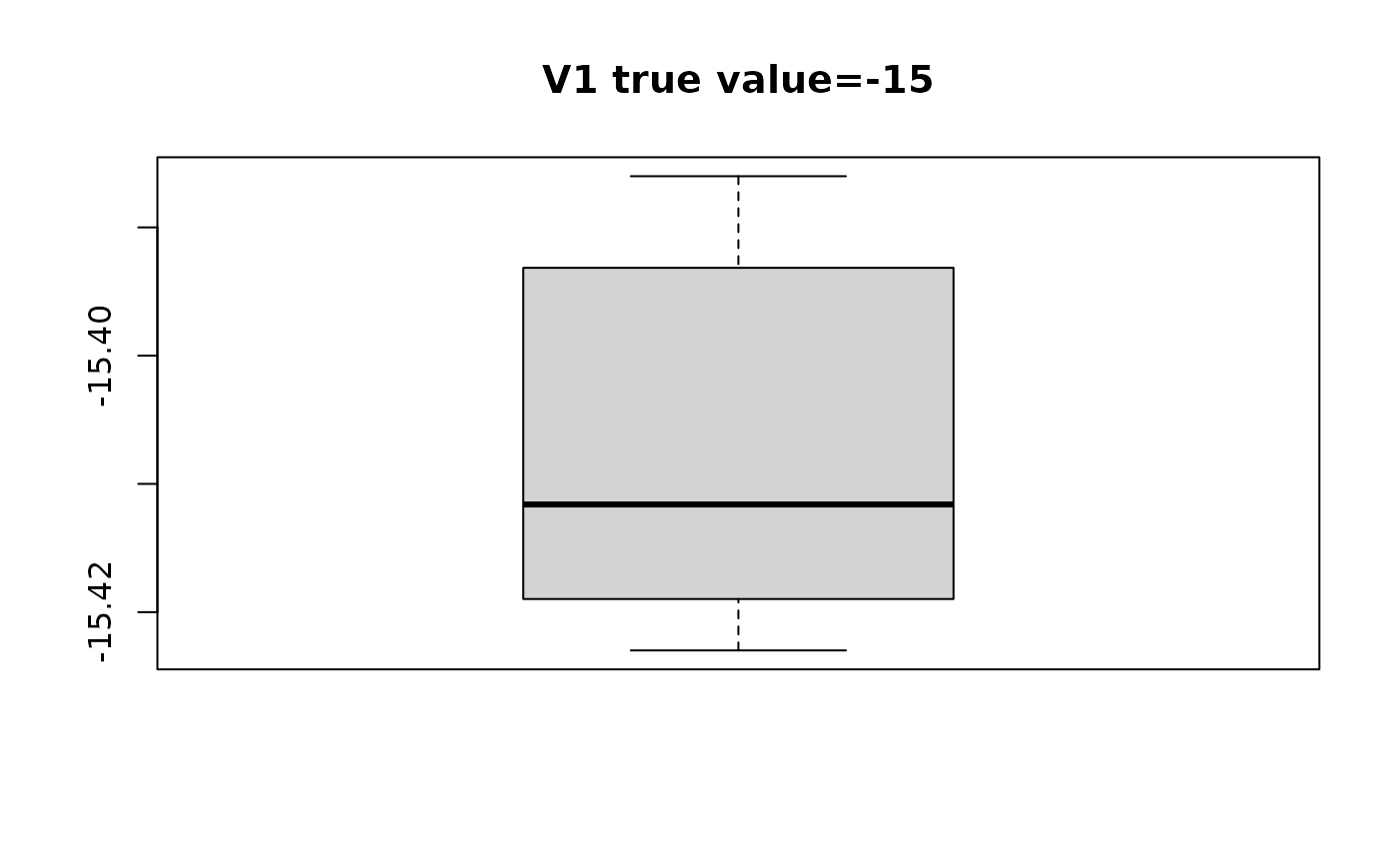
swaglm_summ$lst_estimated_beta_per_variable
#> $V1
#> [1] -15.42298 -15.41904 -15.39433 -15.42253 -15.41751 -15.41548 -15.42189
#> [8] -15.41399 -15.40975 -15.38601 -15.41957 -15.39480 -15.39200 -15.41335
#> [15] -15.41891 -15.40986 -15.39299 -15.38835 -15.38618 -15.39331
#>
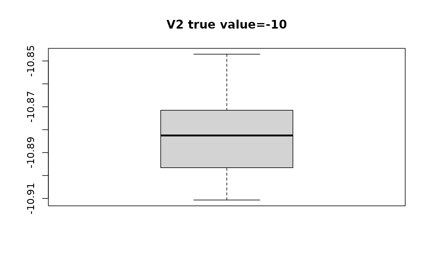
#> $V2
#> [1] -10.88880 -10.91069 -10.87565 -10.85719 -10.87506 -10.88462 -10.88661
#> [8] -10.88503 -10.90536 -10.87101 -10.88042 -10.84705 -10.89722 -10.89594
#> [15] -10.91043 -10.90658 -10.87300 -10.86145 -10.87202 -10.86969
#>
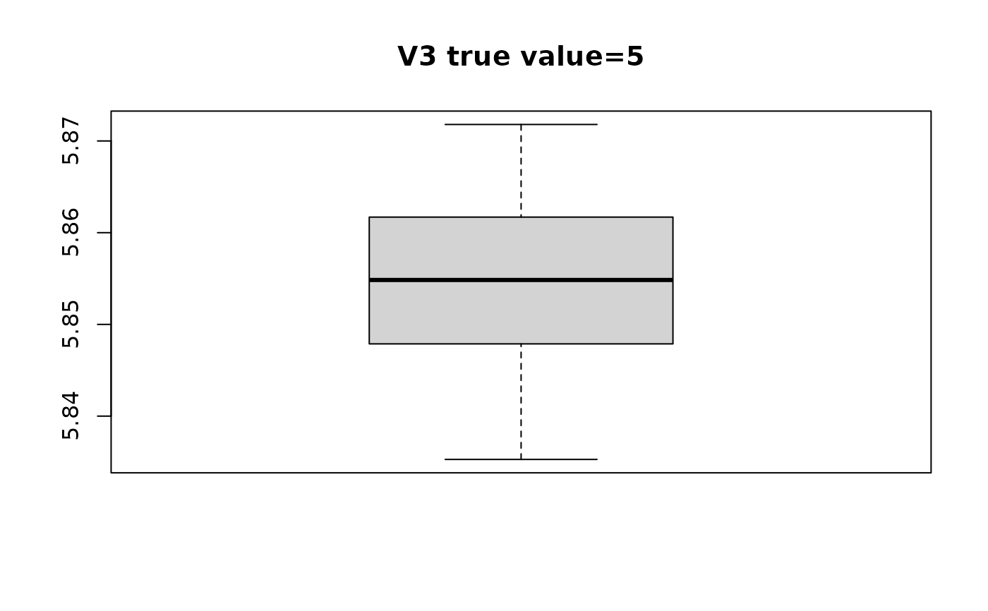
#> $V3
#> [1] 5.866387 5.861586 5.850753 5.853032 5.857510 5.871796 5.865727 5.861812
#> [9] 5.868274 5.856846 5.848506 5.838658 5.847248 5.852137 5.861513 5.856654
#> [17] 5.849975 5.842569 5.846146 5.835279
#>
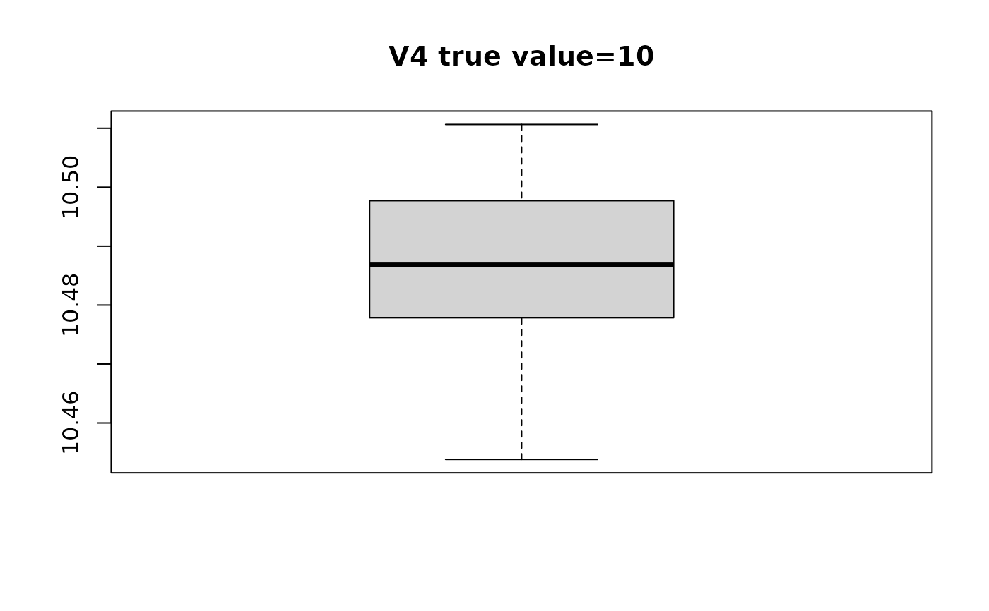
#> $V4
#> [1] 10.50399 10.48690 10.48362 10.50980 10.47527 10.51064 10.50329 10.50079
#> [9] 10.49464 10.49089 10.49341 10.48865 10.46782 10.45853 10.48682 10.48360
#> [17] 10.48279 10.45382 10.48044 10.47352
#>
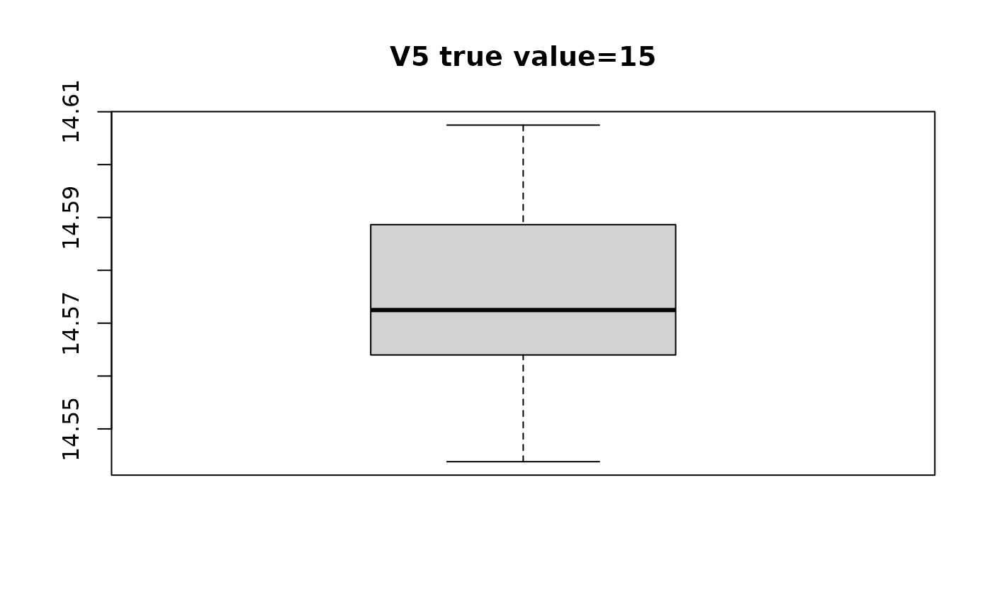
#> $V5
#> [1] 14.56981 14.55198 14.59389 14.58462 14.58305 14.56331 14.56842 14.56537
#> [9] 14.54379 14.58686 14.56654 14.60611 14.57515 14.56466 14.55182 14.54768
#> [17] 14.59224 14.60748 14.59001 14.58728
#>
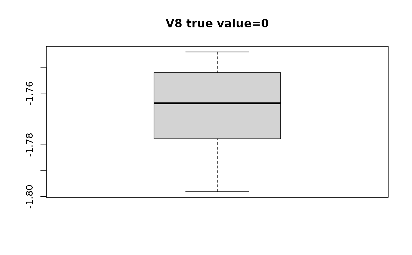
#> $V8
#> [1] -1.757739 -1.779159 -1.751831 -1.776622 -1.749972 -1.754524 -1.758153
#> [8] -1.757246 -1.775884 -1.748051 -1.798152 -1.769693 -1.772099 -1.770955
#> [15] -1.779208 -1.778736 -1.752328 -1.744077 -1.751488 -1.790190
#>
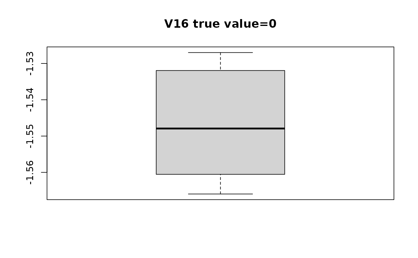
#> $V16
#> [1] -1.548579 -1.564319 -1.531283 -1.543661 -1.548366 -1.546696 -1.547903
#> [8] -1.549986 -1.562112 -1.529190 -1.558967 -1.526998 -1.547935 -1.563234
#> [15] -1.564237 -1.565955 -1.530522 -1.530806 -1.532604 -1.543226
#>
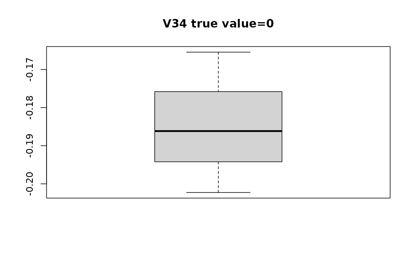
#> $V34
#> [1] -0.1654597 -0.2022687 -0.1861584
#>
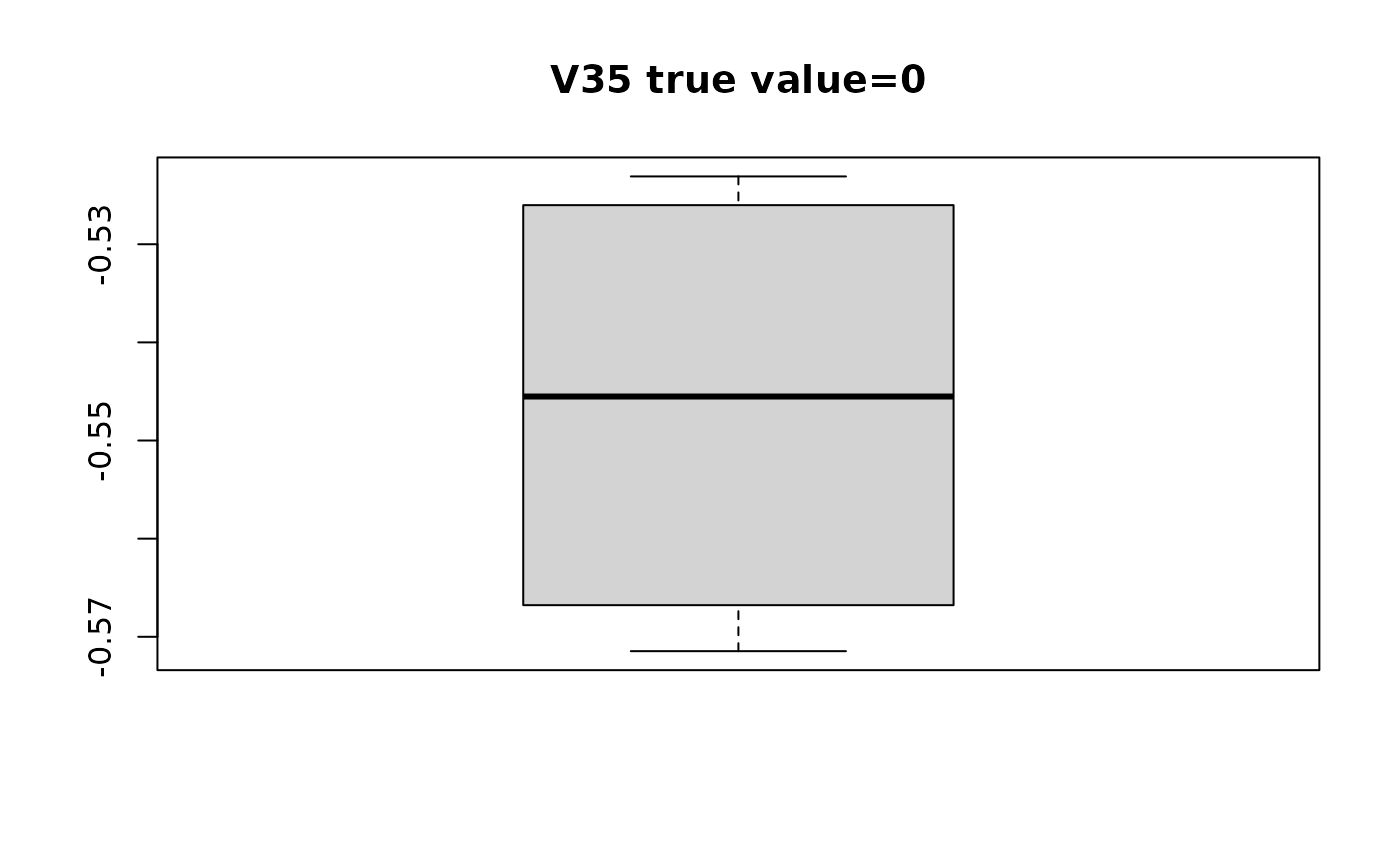
#> $V35
#> [1] -0.5714650 -0.5620896 -0.5289427 -0.5230901
#>
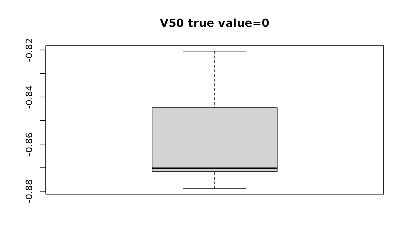
#> $V50
#> [1] -0.8706569 -0.8789415 -0.8650236 -0.8239921 -0.8700605 -0.8704989 -0.8724853
#> [8] -0.8205079
#>
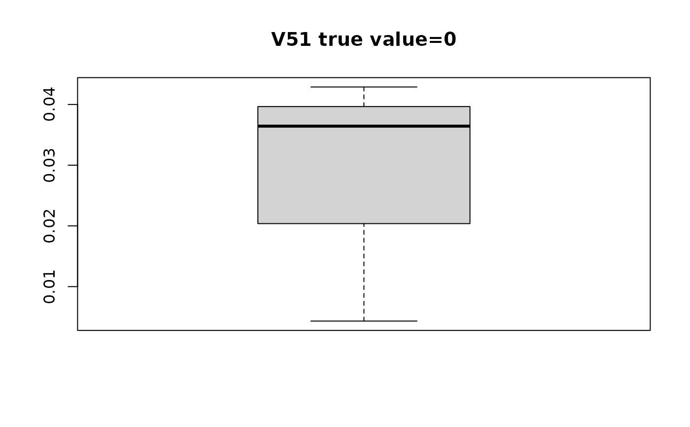
#> $V51
#> [1] 0.036430980 0.004326727 0.042877552
#>
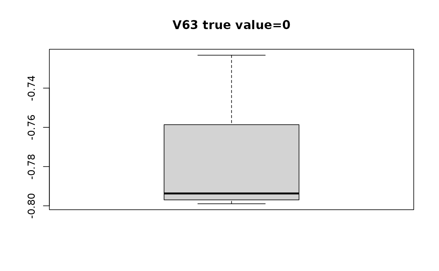
#> $V63
#> [1] -0.7946861 -0.7989666 -0.7698577 -0.7473978 -0.7950032 -0.7989648 -0.7927315
#> [8] -0.7232223
#>
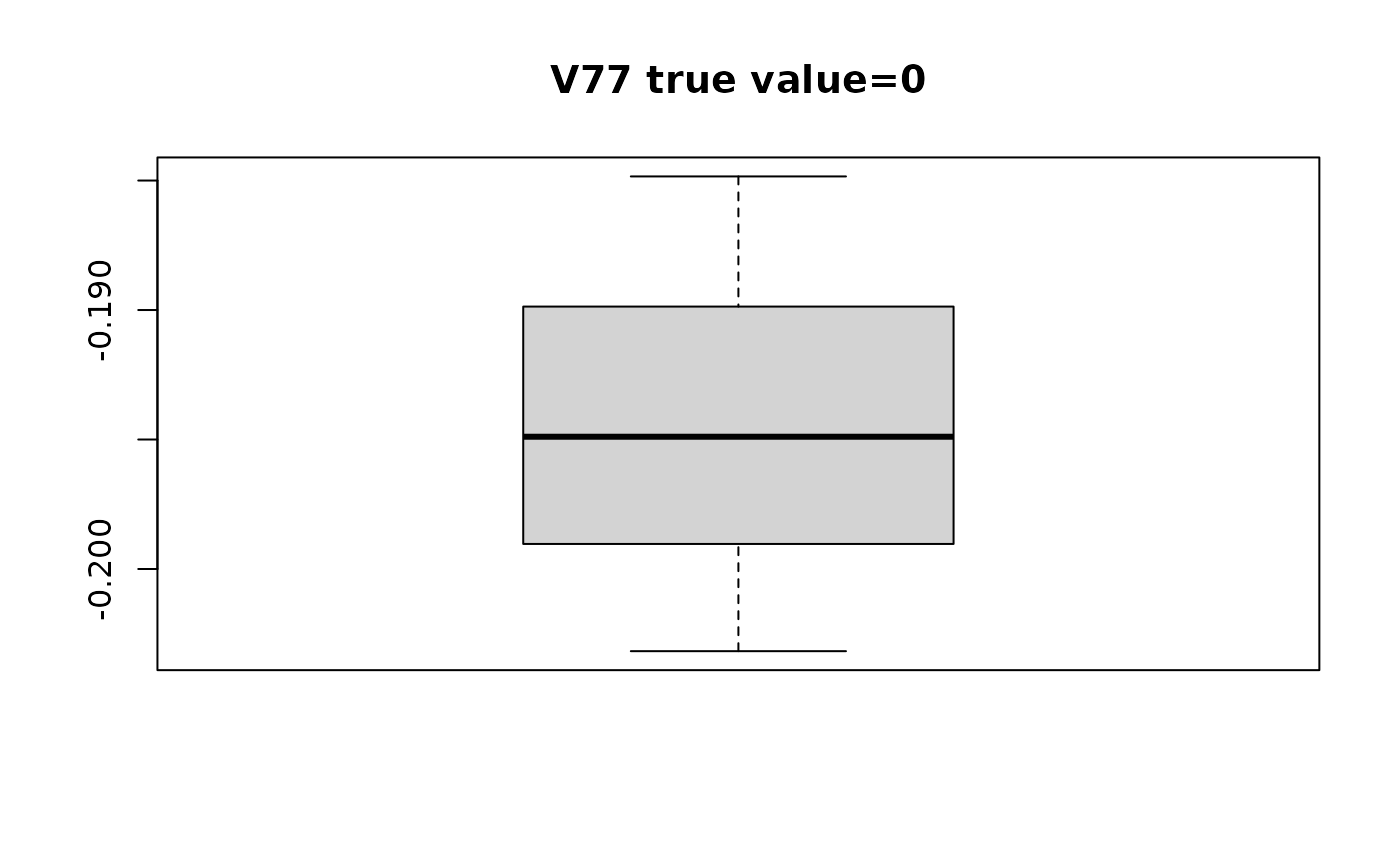
#> $V77
#> [1] -0.1948925 -0.2031730 -0.1848413
#>
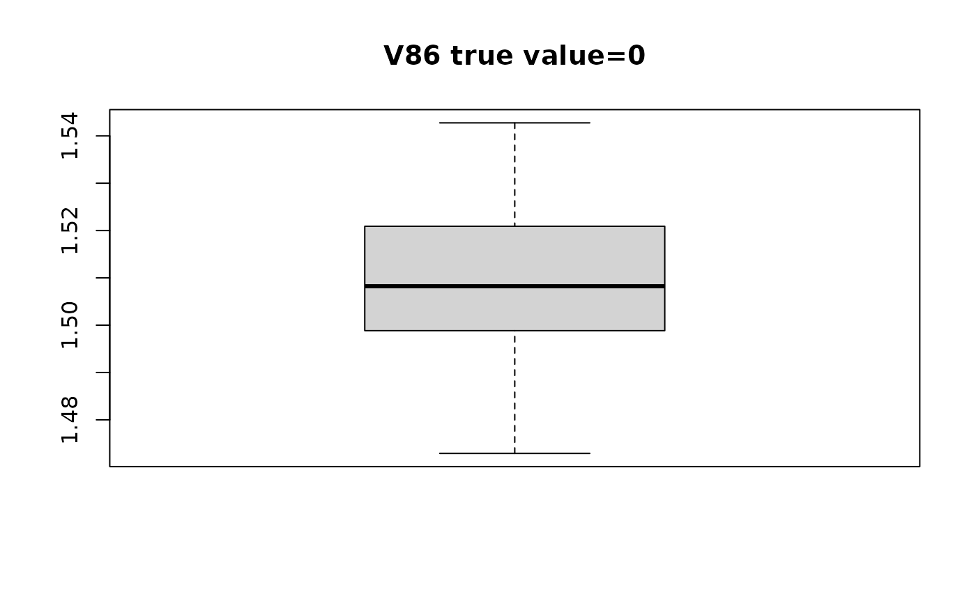
#> $V86
#> [1] 1.529974 1.506564 1.506844 1.515732 1.542760 1.533030 1.529056 1.521742
#> [9] 1.509618 1.510129 1.492906 1.494184 1.485106 1.519009 1.506464 1.498269
#> [17] 1.505715 1.520073 1.499415 1.472900
#>
#> $V95
#> [1] 0.4162630 0.4153874 0.4266401
#>
# plot distribution of estimated beta with respect to true value
for(i in seq_along(swaglm_summ$lst_estimated_beta_per_variable)){
# get variable name
var_name_i = names(swaglm_summ$lst_estimated_beta_per_variable)[i]
var_index_i = as.numeric(substr(var_name_i, 2, nchar(var_name_i)))
boxplot(swaglm_summ$lst_estimated_beta_per_variable[[i]],
main=paste0(var_name_i, " ", "true value=", beta[i]))
}