Graphical User Interface for the Inertial Sensors Calibration
The Generalized Method of Wavelet Moments (GMWM) is a recently proposed statistical approach that allows to estimate the parameters of (complex) time series models in a simple and efficient manner. It is therefore an extremely useful tool to estimate the models underlying the composite processes that characterize the measurement errors of (low-cost) Inertial Measurement Units (IMU). Moreover, aside from efficiently estimating these complex models, the GMWM framework also provides a procedure to select the best model for the data (within a set of given models) based on a prediction-accuracy criterion called the Wavelet Variance Information Criterion (WVIC).
This online platform provides an easy-to-use GUI that allows practitioners to load their calibration data, compare it to the datasheet specifications, identify and estimate potential models as well as select the best candidate among a given set of models.
Installation Instructions
To use the gui4gmwm package, there are currently two options:
Installing through GitHub
The following R packages are also required. Run the following code in an R session and you will be ready to use the development version of gui4gmwm.
# Install dependencies
devtools::install_github("SMAC-Group/gmwm")
devtools::install_github("SMAC-Group/imudata")
install.packages(c("scales", "reshape", "shiny", "shinydashboard", "leaflet"))

# Install the package from GitHub
devtools::install_github("SMAC-Group/gui4gmwm")
Once the gui4gmwm is installed you can run locally the Graphical User Interface (GUI) by using:
library(gui4gmwm)
runApp("gui4gmwm")
Application Guide
Loading calibration data
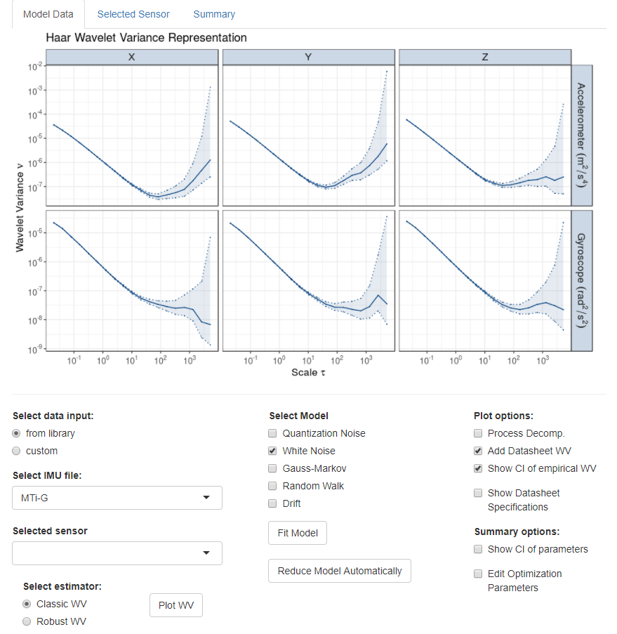
The GMWM GUI presents itself with a Wavelet Variance (WV) log-log plot of a default IMU dataset underneath which the user will find a three column structure where data loading, analysing and modelling options are made available. In the first column there are two buttons that are linked to the two basic ways of loading data in the GUI:
-
From library: the user can select this option to load data from real calibration procedures of different IMUs that can be used to understand how the GMWM GUI works -
Custom: the user can upload a “.txt” file containing calibration data from any inertial sensor
If the user decides to upload data using the “from library” option, then the “Select IMU file” dropdown curtain allows to select the type of IMU that the user intends to calibrate among the datasets available in the GUI. In either case, it is then possible for the user to specify which IMU sensor they intend to analyse and model (e.g. X-axis gyroscope). This can be done by using the second dropdown curtain in which the six different sensors are listed and can consequently be selected.
Plotting the data
The first step towards modelling the error signals that come from an IMU calibration procedure is visualizing the data in a useful manner. As mentioned above, the GUI presents itself with an example of a WV log-log plot of a default IMU calibration dataset. This kind of plot is very commonly used to visualize and identify the type of error signals that characterize IMUs since the form of the WV (similarly to the Allan variance) along with the region in the plot are indicative of the underlying probabilistic models.
According to the selected sensor, it is then possible to select the type of WV that the user wants to plot. More specifically, the default WV is the standard (or classic) WV estimator which is the commonly used one that was proposed by Percival (1995). However, the calibration may be affected by disturbances or forms of contamination which generate outliers in the observed data. This can create considerable bias in the plots and consequent modelling process and is therefore a useful feature to limit this bias in case such a contamination is present. If this is not the case, the standard WV is generally preferrable in terms of statistical efficiency.
Once the choice of the estimator (and the sensor) is made, then the user can click the “Plot / Update WV” button which brings them to the “Selected Sensor” tab where the estimated WV is plotted along with the Confidence Intervals (CI) for the true WV. As mentioned before, this plot can then be used to understand the possible underlying models that characterize the error signal.
Plotting options
There are a few options available to the user in order to add/remove features to the estimated WV plot. These can be found in the first part of the third column (“Options”) of the GMWM GUI under “Plot options”. The only arguments that are of interest when simply plotting the estimated WV are two (we will discuss the third argument further below)
-
Include CI for WV: this argument is ticked by default and allows to visualize the CI for the true WV, meaning the range of values (for each scale of WV) within which there is a 95% probability of finding the true WV; -
Overlay Datasheet Specifications: this argument allows to visualize the WV implied by the noise model given by the supplier. In this case, these models are those given for the datasets already available in the GUI (and that can be chosen using the “from library” option) and in all cases the noise model is a White Noise with a corresponding value for the innovation variance \(\sigma^2\).
Modelling using the GMWM
Once the user has identified a possible set of models that could adequately describe the observed WV, it is then possible to estimate the parameters of these models. This step is carried out in the second column of the GMWM GUI under “GMWM Modelling” which makes available a set of five noise models that can be combined in different ways to build a large variety of composite models that characterize IMU error signals. Four of these noise models can only be included once within a composite model while the fifth noise model is the Gauss-Markov noise model which can theoretically be included any finite number of times. However, in practice it is extremely rare to go beyond five Gauss-Markov models within a general composite model. Hence, when a Gauss-Markov model is selected by ticking the corresponding button, a slider appears in the GUI allowing the user to specify how many Gauss-Markov processes they want to include in the overall model (by default one which can then go up to five).
Once a model is specified it is possible to obtain an expression for the WV implied by the chosen (composite) model which we denote as \(\mathbf{\nu}(\mathbf{\theta})\) where \(\mathbf{\nu}\) represents the true WV and \(\mathbf{\theta}\) represents the model parameter vector which we are interested in estimating. Based on this, the GMWM is defined as the result of the following generalized least-squares optimization problem
\[\hat{\mathbf{\theta}} = \underset{\mathbf{\theta}}{\text{argmin}}\,(\hat{\mathbf{\nu}} - \mathbf{\nu}(\mathbf{\theta}))^T\Omega(\hat{\mathbf{\nu}} - \mathbf{\nu}(\mathbf{\theta}))\]
where \(\hat{\mathbf{\nu}}\) represents the estimated WV (standard or robust) and \(\Omega\) represents a weighting matrix that depends on the variance of the estimator \(\hat{\mathbf{\nu}}\) (see Guerrier et al., 2013).
Once the model is specified (by ticking the corresponding buttons), in order to obtain the estimated parameter vector \(\hat{\mathbf{\theta}}\) of interest the GMWM GUI provides the “Fit Model” button. By using this option the GUI starts the estimation procedure in the R statistical enviroment and outputs the results that are presented in two different ways:
-
WV visual fit: the WV implied by the estimated model (i.e. \(\mathbf{\nu}(\hat{\mathbf{\theta}})\)) is plotted against the previous estimated WV plot. This tool allows the user to visually assess whether the estimated model appears to well describe the observed WV coming from the data. By default the WV plot also shows the WV implied by each individual noise model which contributes to the overall WV. In this manner it is possible to understand if the presence of a specific noise model is needed or not. However, this plotting option can be removed by ticking the “Process Decomp.” button which represents the third argument in the “Plot options” area discussed earlier on. NB When the fitted WV is plotted it is not possible to also plot the noise model implied by the datasheet specifications. -
Summary output: the numerical values of the estimated parameters \(\hat{\mathbf{\theta}}\) are given in the “Summary” tab of the GUI. Another information that is given is the value of the GMWM objective function given earlier which has to be minimized. As a general rule, the smaller the value then the better the model fits the observed data. However this may not necessarily be the goal to pursue as explained further on.
Summary options
As for the plotting features, obtaining the summary of the estimation procedure also has available options that are included in the “Summary options” section. There are two arguments available:
-
Include CI for Parameters: if the button linked to this option is ticked, then aside from the value of the estimated model parameters the user will also obtain the values of the 95% CI for each parameter. -
Edit Optimization Parameters: when selecting this option the user will be offered additional arguments which allow them to modify some features used to find starting values for the optimization process to run. -
Number of Simu. for Starting Values: this argument allows to modify the number of simulated starting values that are evaluated at the objective function. The set of simulated starting values that minimize the objective function are then used as starting values for the optimization procedure. The larger the number of simulated starting values then larger is the probability of finding starting values that allow to get closer to the true minimum of the objective function. The drawback of increasing this number however lies in the fact that the overall estimation procedure experiences a comparable decrease in computational speed. -
Simulation seed: this argument controls the seed that determines the random value generation process for the starting values which in turn affect the optimization process. This is mainly used to ensure replicability of the estimation procedure.
Automatically Selecting the Model
A final option that’s available to the GMWM GUI user consists in the “Reduce Model Automatically” feature also included under the “GMWM Modelling” section in the second column. In this case, the user can specify a general composite model in which they think all the potential models for the observed error signal are included. For example, after observing the WV plot the user may believe that the most complex model that could fit the observed WV would be a model composed by a White Noise plus a Random Walk. In this case they select the latter model using the options explained earlier in the second column for the GMWM estimation and then click the “Reduce Model Automatically” button which uses the WVIC to select the “best” model among the possible candidates (in the case of the considered example there would be three candidates: White Noise, Random Walk, White Noise plus Random Walk).
The WVIC is a model selection criterion (Guerrier et al., 2017) which provides a consistent estimator of the out-of-sample prediction error of a model in terms of its WV. More specifically, the WVIC estimates the prediction error of a model when predicting future values of the WV when computed on other samples of the error signal issued from the same IMU. Hence, we would want to select a model that minimizes this error and this does not necessrily correspond to the model that minimizes the objective function on the observed sample (which in general is achieved by choosing the most complex model possible). The WVIC therefore provides a balance between model complexity and out-of-sample variability in terms of prediction, penalizing models that are overly complex for the observed data.